Introduction & Background
Overview
Welcome to Modeling with Linear & Generalized Linear Models! In this first module we will:
- Review the notation and basic statistical concepts that will recur throughout the course.
- Introduce our running motivating example: predicting house prices using regression.
By the end of this lesson you should feel comfortable with symbols like \(Y\), \(X\), \(a\), and be ready to formulate and fit your first linear model.
Notation
Throughout the course we will use the following conventions:
| Symbol | Meaning |
|---|---|
| \(n\) | Number of observations (data points) |
| \(p\) | Number of predictors (features) including intercept |
| \(X_i\) or \(x_i\) | Features (predictors) for observation \(i\) |
| \(Y_i\) or \(y_i\) | The response (target) for observation \(i\) |
| \(X\) | The \(n\times p\) design matrix |
| \(a\) or \(a_j\) | Model coefficients (slope, intercept) |
| \(\varepsilon_i\) | Random error term for observation \(i\) |
| \(\bar{X}\), \(\bar{Y}\) | Sample means for random variables |
| \(s^2\) | Sample variance |
Before fitting models, let’s recall some foundational ideas:
Random Variables & Expectations
- A random variable \(Y\) has a probability distribution.
- The expected value (mean) is
\[ \mathbb{E}[Y] = \mu = \int y\,dF_Y(y) \] - The variance measures spread:
\[ \mathrm{Var}(Y) = \mathbb{E}\bigl[(Y - \mu)^2\bigr] = \sigma^2. \]
Sampling & Estimation
- The sample mean of \(y_1,\dots,y_n\): \[ \bar y = \frac1n\sum_{i=1}^n y_i. \]
- The sample variance: \[ s^2 = \frac{1}{n-1}\sum_{i=1}^n (y_i - \bar y)^2. \]
Covariance & Correlation
- Covariance of two random variables \(X\) and \(Y\): \[ \mathrm{Cov}(X,Y) = \mathbb{E}\bigl[(X - \mathbb{E}[X])(Y - \mathbb{E}[Y])\bigr]. \]
- Correlation (Pearson’s \(\rho\)) is the standardized covariance: \[ \rho_{XY} = \frac{\mathrm{Cov}(X,Y)}{\sqrt{\mathrm{Var}(X)\,\mathrm{Var}(Y)}}. \]
We will see how these quantities enter into formulas for parameter estimates, tests, and confidence intervals.
Motivating Example: House Price Prediction
To ground our discussion, we’ll work throughout the course with a real-world dataset of house sales. Our goal:
Predict the sale price \(y\) of a home from features such as:
- Size (\(\text{sqft}\))
- Number of bedrooms
- Age of the home
- Neighborhood quality (that will be encoded as dummy variables)
In notation:
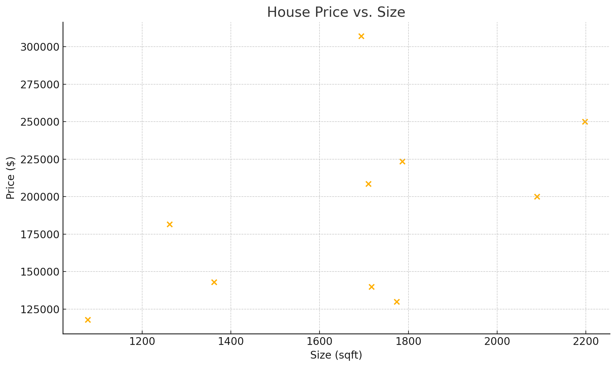
\[ y_i \;=\; a_0 + a_1\,\text{sqft}_i + a_2\,\text{beds}_i + a_3\,\text{age}_i + \cdots + \varepsilon_i. \]Here is a sample of 10 lines:
| Size | Number of bedrooms | Age | Neighborhood | Price |
|---|---|---|---|---|
| 1710 | 3 | 5 | CollgCr | 208500 |
| 1262 | 3 | 31 | Veenker | 181500 |
| 1786 | 3 | 7 | CollgCr | 223500 |
| 1717 | 3 | 91 | Crawfor | 140000 |
| 2198 | 4 | 8 | NoRidge | 250000 |
| 1362 | 1 | 16 | Mitchel | 143000 |
| 1694 | 3 | 3 | Somerst | 307000 |
| 2090 | 3 | 36 | NWAmes | 200000 |
| 1774 | 2 | 77 | OldTown | 129900 |
| 1077 | 2 | 69 | BrkSide | 118000 |
Here’s your scatter plot of Price (y) vs. Size (x):
Later modules will show how to:
- Estimate the coefficients \(a\) (Ordinary Least Squares)
- Test hypotheses about feature effects (t-tests, F-tests)
- Check model assumptions (residual diagnostics)
- Extend to generalized linear models (e.g., logistic regression)
With our notation and basic statistics clear, we’re ready to dive in to Simple Linear Regression in the next lesson!