Single Neuron and Loss
The Perceptron as a Building Block
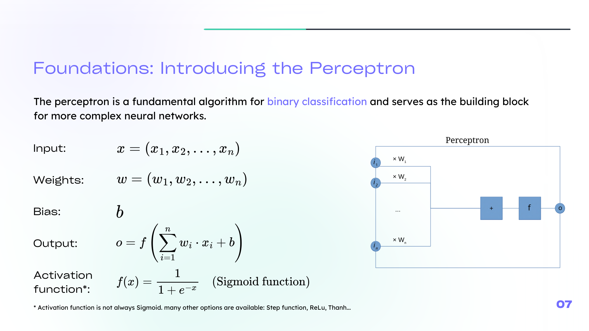
The perceptron is one of the earliest neural models for binary classification. It takes an input vector \(x\), combines it linearly with weights \(w\), adds a bias \(b\), then applies an activation function:
\[ z = w^T x + b \]\[ a = g(z) \]This simple structure is the building block of much larger networks.
Perceptron Versus Logistic Regression
A useful bridge from classical machine learning is logistic regression. In a neural-network view, logistic regression can be seen as a single neuron whose activation is the sigmoid function.
The sigmoid maps any real number into a probability-like value:
\[ \sigma(z) = \frac{1}{1 + e^{-z}} \]The related logit transform goes in the other direction:
\[ \mathrm{logit}(p) = \log\left(\frac{p}{1-p}\right) \]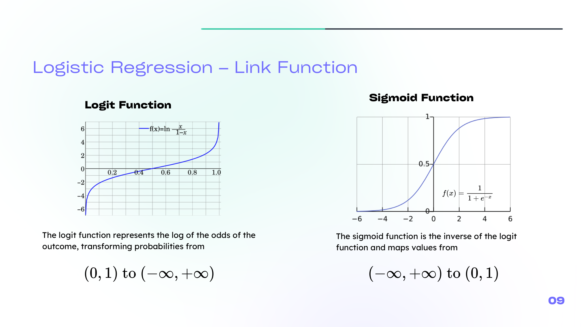
This is a helpful intuition: many neural-network ideas start by extending what we already know from logistic regression.
Loss, Cost, and Cross-Entropy
To train a model, we need a way to measure how wrong it is.
- A loss measures the error for one example.
- A cost aggregates that error over the dataset.
For classification, one of the most important choices is cross-entropy, which matches the probabilistic interpretation of logistic outputs.
For binary targets \(y \in \{0,1\}\), the average logistic cost is:
\[ J(w,b) = -\frac{1}{m}\sum_{i=1}^{m} \left[ y^{(i)} \log a^{(i)} + (1-y^{(i)}) \log(1-a^{(i)}) \right] \]This cost is equivalent to the negative log-likelihood under a Bernoulli model.
Gradient Descent
Once the cost is defined, we minimize it by updating parameters in the opposite direction of the gradient:
\[ w \leftarrow w - \alpha \frac{\partial J}{\partial w}, \qquad b \leftarrow b - \alpha \frac{\partial J}{\partial b} \]where \(\alpha\) is the learning rate.
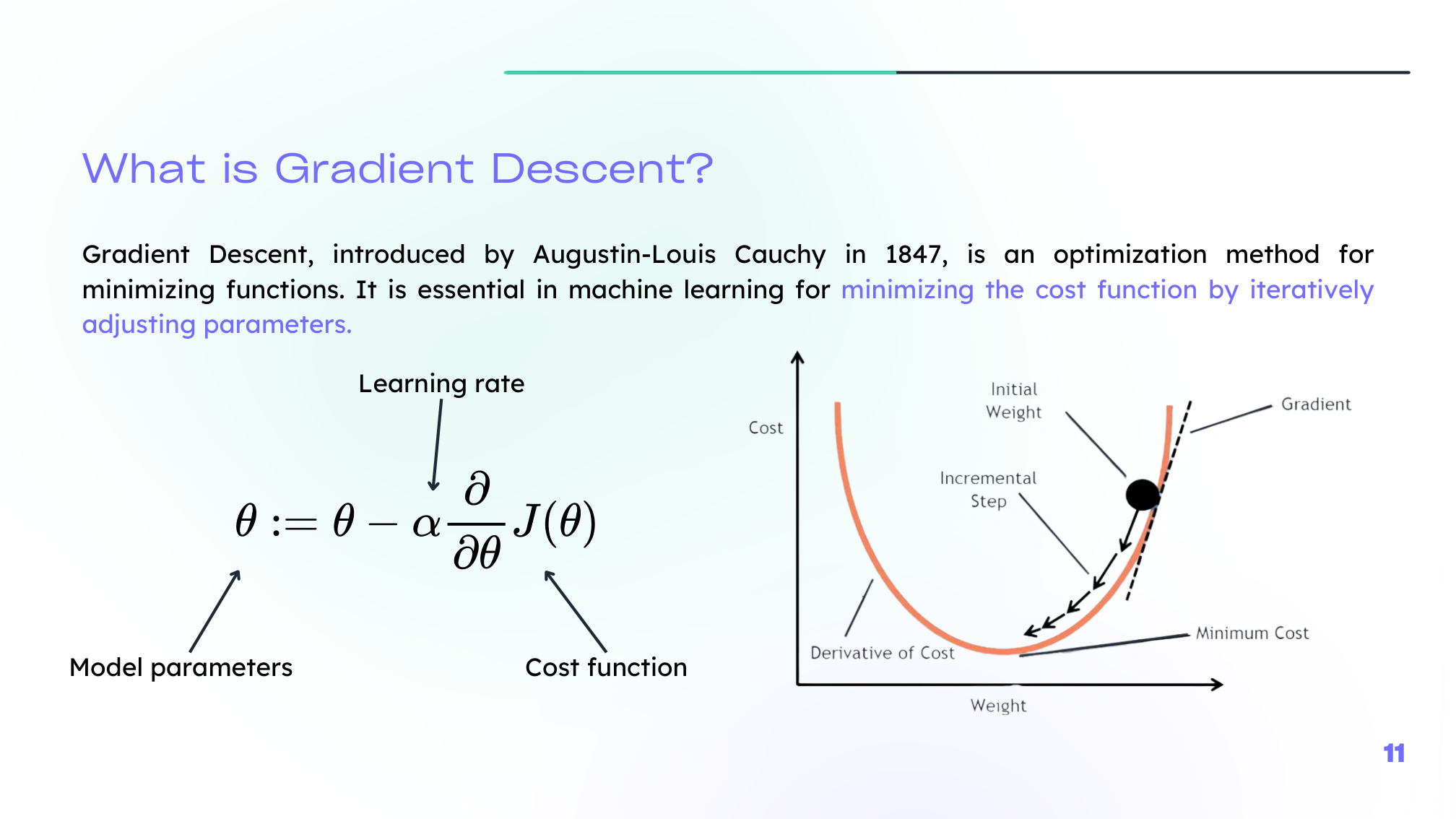
The learning rate controls the step size:
- too small, and learning is slow,
- too large, and training can become unstable.
Summary
In this lesson we covered:
- The perceptron as the simplest neural building block
- The linear combination \(z = w^T x + b\)
- The sigmoid neuron as a neural view of logistic regression
- The difference between loss and cost
- Cross-entropy for binary classification
- Gradient descent as the main optimization mechanism
Next: We will connect many neurons together and see how forward propagation and backpropagation make learning possible.