Multiple Regression and Feature Engineering
Multiple Regression
The multiple regression model relates more than one predictor to a single response variable.
For \(p\) predictors plus an intercept, the model is:
\[ Y = a_0 + a_1 X_1 + a_2 X_2 + \ldots + a_p X_p + \varepsilon \]where:
- \(Y\) is the target variable
- \(X_1, X_2, \ldots, X_p\) are the predictors
- \(a_0, a_1, \ldots, a_p\) are the coefficients
- \(\varepsilon\) is the error term
For a single observation, we can write:
\[ y = (x_1, x_2, \ldots, x_p) \begin{pmatrix} a_1 \\ a_2 \\ \vdots \\ a_p \end{pmatrix} + \varepsilon \]Matrix Notation
For a sample of \(n\) observations, we use matrix notation to represent the model compactly.
The Design Matrix
The full model can be written as:
\[ \begin{aligned} \begin{pmatrix} y_1 \\ y_2 \\ y_3 \\ \vdots \\ y_n \end{pmatrix} &= \begin{pmatrix} x_{11} & x_{12} & \cdots & x_{1p} \\ x_{21} & x_{22} & \cdots & x_{2p} \\ x_{31} & x_{32} & \cdots & x_{3p} \\ \vdots & \vdots & \ddots & \vdots \\ x_{n1} & x_{n2} & \cdots & x_{np} \end{pmatrix} \begin{pmatrix} a_1 \\ a_2 \\ a_3 \\ \vdots \\ a_p \end{pmatrix} + \begin{pmatrix} \varepsilon_1 \\ \varepsilon_2 \\ \varepsilon_3 \\ \vdots \\ \varepsilon_n \end{pmatrix} \end{aligned} \]Where:
- Response vector \(Y\): \(n \times 1\) matrix containing all observed responses
- Design matrix \(X\): \(n \times p\) matrix of predictor values
- Coefficient vector \(a\): \(p \times 1\) matrix of parameters to estimate
- Error vector \(E\): \(n \times 1\) matrix of random errors
In compact form:
\[ Y = Xa + E \]For regression with intercept, we set the first element of each row to 1:
\[ x_{i1} = 1 \quad \forall i \]This allows the intercept \(a_0\) to be included as the first coefficient.
Matrix Operations Review
Matrix Multiplication
The product of an \(m \times n\) matrix \(A\) and an \(n \times p\) matrix \(B\) is an \(m \times p\) matrix \(C\):
\[ C_{ij} = \sum_{k=1}^{n} A_{ik} B_{kj} \]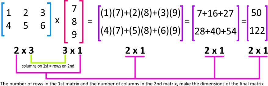
Example:
\[ \begin{aligned} \begin{pmatrix} 1 & 2 & 3 \\ 4 & 5 & 6 \end{pmatrix} \begin{pmatrix} 7 \\ 8 \\ 9 \end{pmatrix} &= \begin{pmatrix} (1)(7)+(2)(8)+(3)(9) \\ (4)(7)+(5)(8)+(6)(9) \end{pmatrix} \\ &= \begin{pmatrix} 50 \\ 122 \end{pmatrix} \end{aligned} \]Matrix Transpose
The transpose \(A^T\) of a matrix \(A\) is obtained by flipping rows and columns:
\[ (A^T)_{ij} = A_{ji} \]Example:
\[ \begin{aligned} \begin{pmatrix} 1 & 2 & 3 & 4 \\ 5 & 6 & 7 & 8 \\ 9 & 10 & 11 & 12 \end{pmatrix}^{\mathsf T} &= \begin{pmatrix} 1 & 5 & 9 \\ 2 & 6 & 10 \\ 3 & 7 & 11 \\ 4 & 8 & 12 \end{pmatrix} \end{aligned} \]Matrix Inverse
A matrix \(B\) is the inverse of \(A\) if:
\[ B \cdot A = A \cdot B = I_n \]where \(I_n\) is the \(n \times n\) identity matrix.
Notation: \(B = A^{-1}\)
Important properties:
- Only square matrices can have an inverse
- A matrix that is not invertible is called singular or degenerate
- A matrix is invertible if it has full column rank \(n\) (no perfect multicollinearity)
Application to solving systems:
\[ AX = Y \quad \Leftrightarrow \quad X = A^{-1}Y \]Norm of a Vector
The Euclidean norm (or \(\ell_2\)-norm) of a vector \(v\) is:
\[ \|v\|^2 = v^T v = v_1^2 + v_2^2 + \ldots + v_p^2 \]Example:
For \(v = \begin{pmatrix} -1 \\ -2 \\ 3 \\ 4 \end{pmatrix}\):
\[ \|v\| = \sqrt{(-1)^2 + (-2)^2 + 3^2 + 4^2} = \sqrt{1 + 4 + 9 + 16} = \sqrt{30} \]Ordinary Least Squares (OLS) in Matrix Form
We need to find the vector \(a\) that minimizes:
\[ \sum_{i=1}^{n} (y_i - \hat{y}_i)^2 = \sum_{i=1}^{n} \left( y_i - \sum_{j=1}^{p} a_j x_{ij} \right)^2 = \|Y - X \cdot a\|^2 \]Normal Equation
The analytical solution for OLS is given by the normal equation:
\[ \hat{a} = (X^T X)^{-1} X^T Y \]Assumptions:
- \(X\) has full column rank: \(\text{rank}(X) = p\)
- This ensures \(X^T X\) is invertible
- Equivalently: \(\text{rank}(X^T X) = \text{rank}(XX^T) = \text{rank}(X)\)
When Normal Equation Fails
The normal equation cannot be used if:
-
Perfect multicollinearity: One predictor is a linear combination of others
- Example: \(X_3 = 2X_1 + 3X_2\)
- Result: Parameters are non-identifiable (no unique solution)
-
Too few observations: \(n < p\)
- Fewer data points than parameters to estimate
- \(\text{rank}(X) \leq \min(n, p)\)
Note: If predictors are highly but not perfectly correlated, \(X^T X\) is technically invertible, but the inverse is numerically unstable. This reduces the precision of parameter estimates and inflates standard errors.
Binary and Categorical Variables
Dummy Variables
Dummy variables are binary (0/1) variables that encode group membership.
Example: Binary Feature
- House has a garden:
garden = 1 - House doesn't have a garden:
garden = 0
Encoding Categorical Variables
For a categorical variable with \(K\) categories, create \(K-1\) dummy variables.
Example: Foundation Type
Suppose Foundation has 5 categories: Brick, Cinder Block, Slab, Stone, Wood.
Create 4 dummy variables:
Foundation_CinderBlock: 1 if Cinder Block, 0 otherwiseFoundation_Slab: 1 if Slab, 0 otherwiseFoundation_Stone: 1 if Stone, 0 otherwiseFoundation_Wood: 1 if Wood, 0 otherwise
Reference category: Brick (when all dummies are 0)
The coefficient for each dummy represents the difference in mean response compared to the reference category, holding other variables constant.
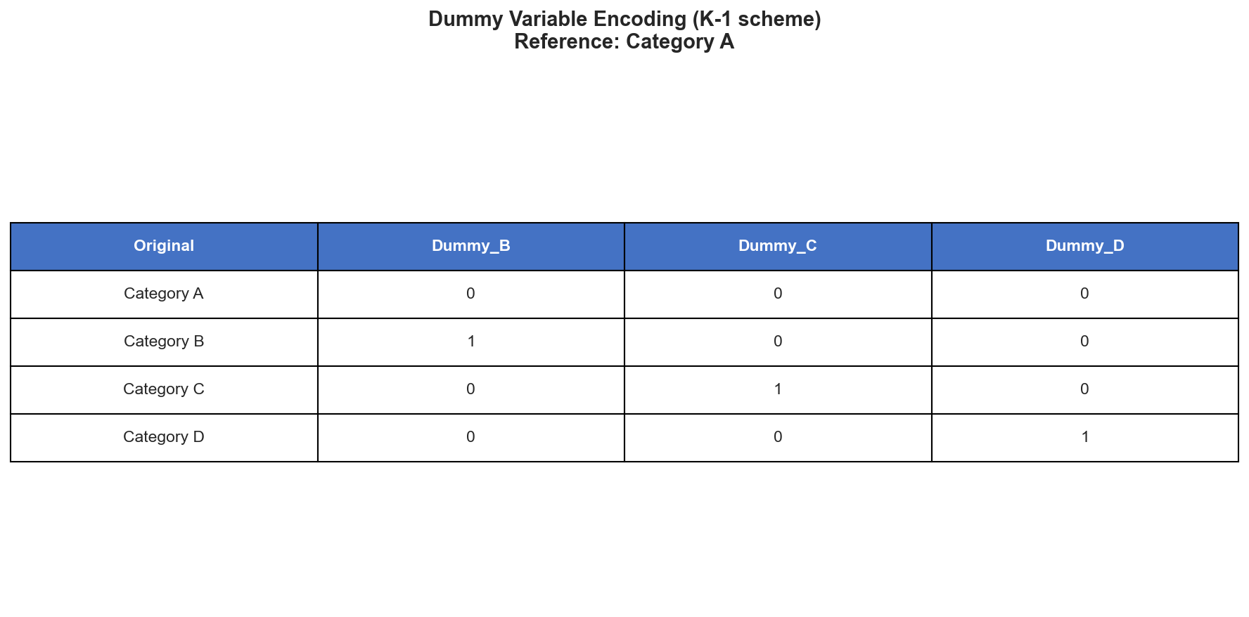
Why \(K-1\) and not \(K\)? Including all \(K\) dummies would create perfect multicollinearity with the intercept, making \(X^T X\) singular.
Predictor Transformations and Interactions
Feature engineering is the creation of new predictors by applying transformations to the original variables.
Common Transformations
\[ f_1(X) = \sqrt{x_1} \qquad f_2(X) = \log(x_2) \qquad f_3(X) = \sin(x_3) \]Benefits:
- Capture nonlinear relationships
- Improve model fit
- Address skewness or non-constant variance in predictors
Interaction Terms
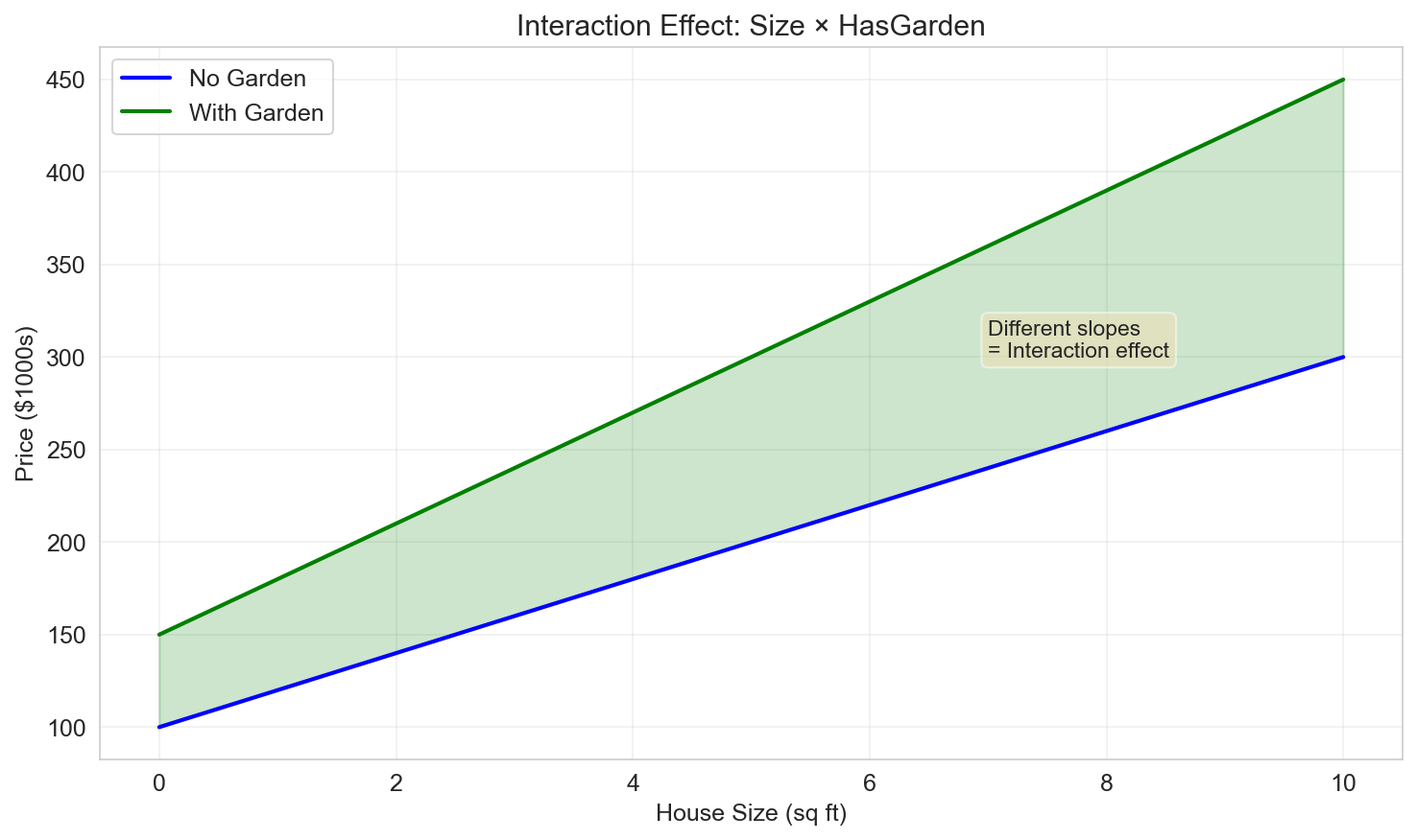
An interaction between two variables captures how the effect of one variable depends on the level of another.
\[ f(X) = x_1 \times x_2 \]Example:
\[ Y = a_0 + a_1 \, \text{Size} + a_2 \, \text{HasGarden} + a_3 \, (\text{Size} \times \text{HasGarden}) + \varepsilon \]The coefficient \(a_3\) tells us how much the effect of Size on Price changes when the house has a garden.
Polynomial Regression
Polynomial regression is a special case of multiple linear regression using power functions as transformations:
\[ f_k(x) = x^k \]For a polynomial of degree \(p\):
\[ Y = a_0 + a_1 x + a_2 x^2 + \ldots + a_p x^p + \varepsilon \]Key point: Although the model is nonlinear in \(x\), it is still linear in the parameters \(a_0, a_1, \ldots, a_p\), so we can use OLS.
Example: Quadratic Fit
\[ Y = a_0 + a_1 x + a_2 x^2 + \varepsilon \]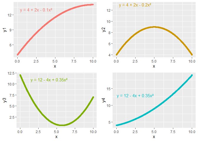
Warning: High-degree polynomials can lead to overfitting. Always validate on held-out data.
Summary
In this lesson we covered:
- ✅ Multiple regression with multiple predictors
- ✅ Matrix notation and the design matrix
- ✅ Matrix operations (multiplication, transpose, inverse, norms)
- ✅ Normal equation for solving OLS
- ✅ Dummy variables for categorical predictors
- ✅ Feature engineering: transformations and interactions
- ✅ Polynomial regression for nonlinear relationships
Next: We'll explore model selection and regularization — hypothesis testing for coefficients, choosing the best predictors, dealing with collinearity, and regularization techniques like Ridge and Lasso.