Forward, Backpropagation, and Activation Functions
From One Neuron to a Network
Once we stack neurons into layers, we move from a single decision boundary to a model that can learn much richer transformations.
In a shallow network, we usually distinguish:
- an input layer,
- one or more hidden layers,
- an output layer.
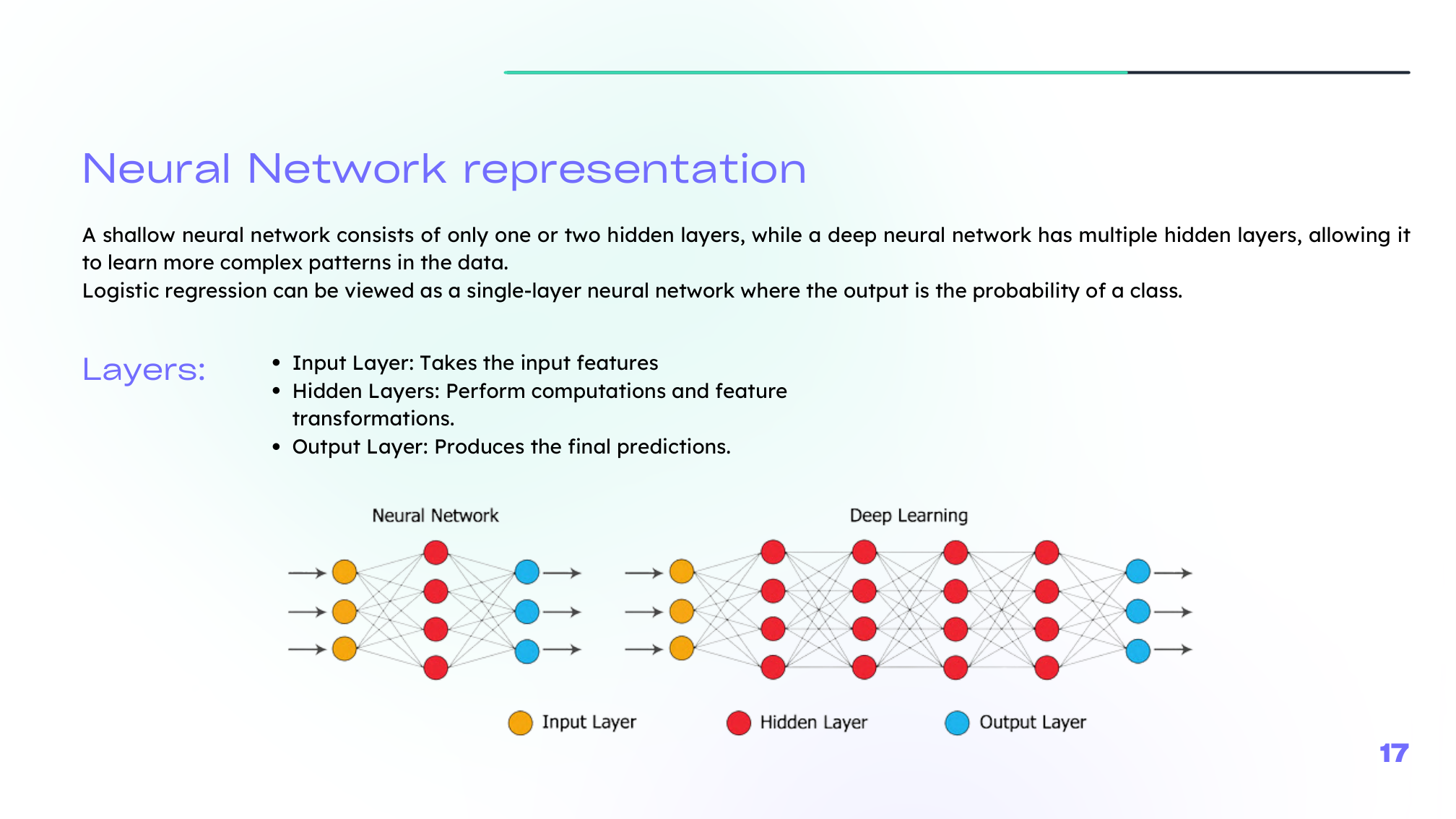
Deep networks simply repeat this pattern with more hidden layers.
Forward Propagation
Forward propagation computes the prediction layer by layer.
For layer \(l\):
\[ Z^{[l]} = W^{[l]} A^{[l-1]} + b^{[l]} \]\[ A^{[l]} = g^{[l]}(Z^{[l]}) \]So each layer performs:
- a linear transformation,
- followed by a nonlinear activation.
Vectorization is essential here. Instead of processing one example at a time, we compute many examples in parallel using matrix operations.
Backpropagation
Backpropagation applies the chain rule to compute how the loss changes with respect to each parameter in the network.
The logic is:
- compute the output error,
- move backward through the layers,
- accumulate gradients for each \(W^{[l]}\) and \(b^{[l]}\),
- update parameters with gradient descent.
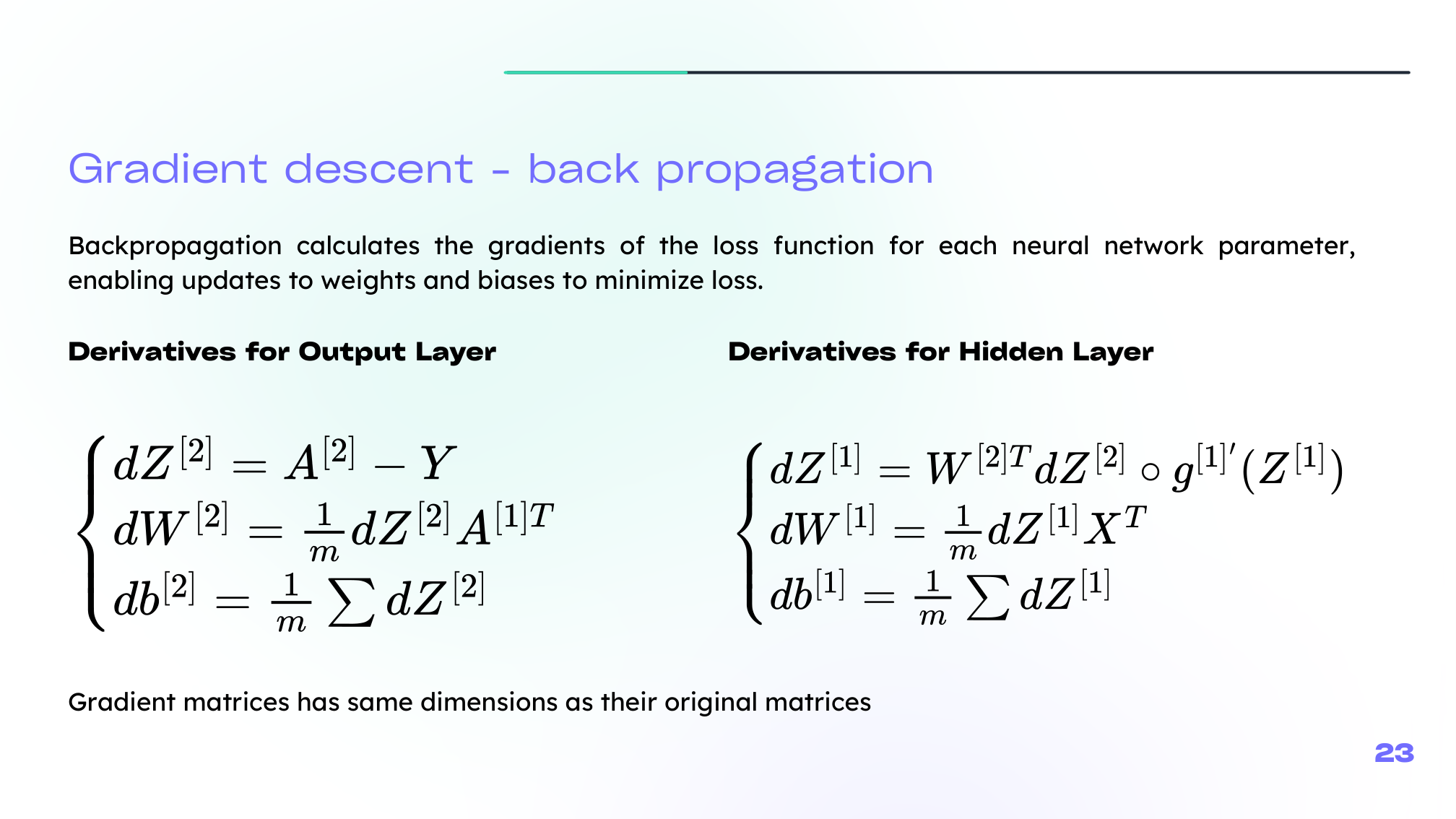
This is the engine that makes neural networks trainable.
Activation Functions
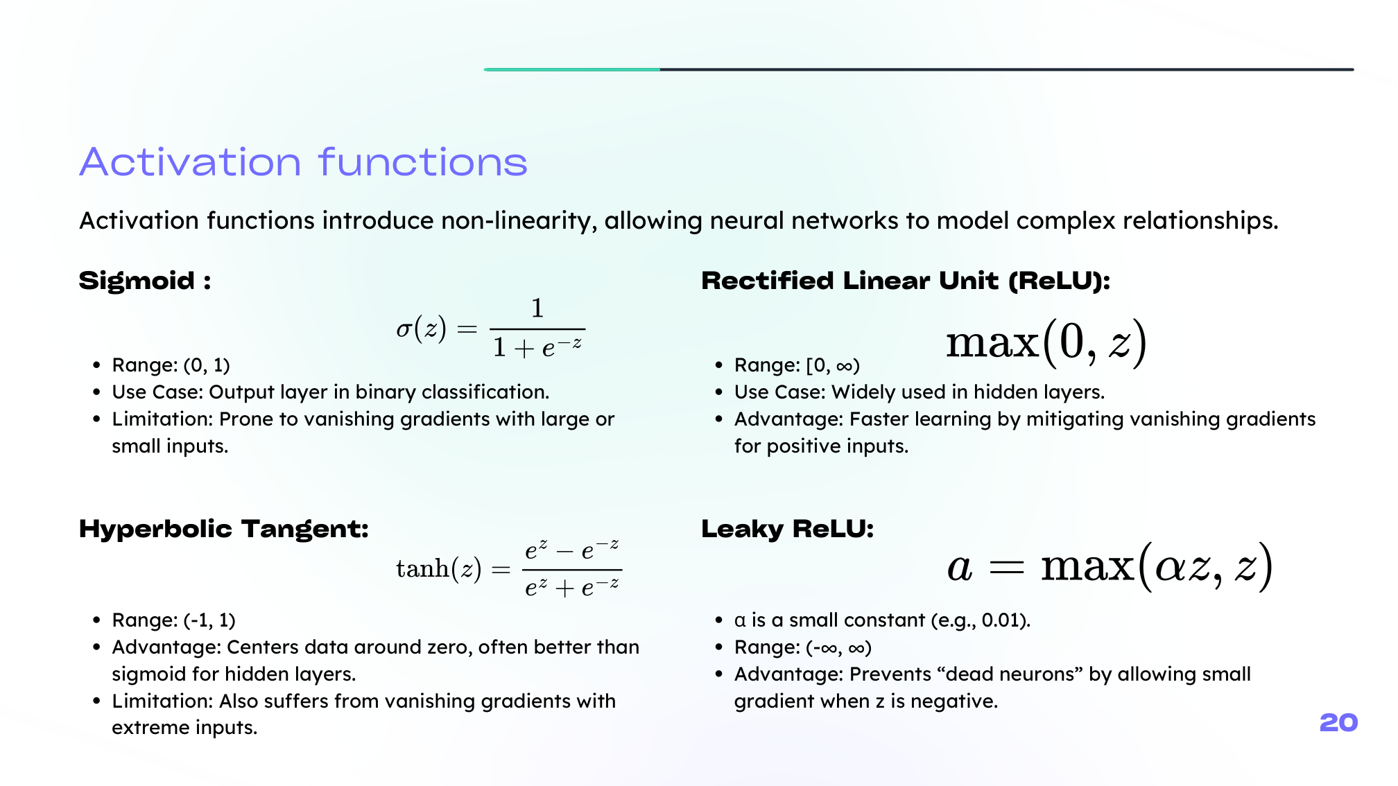
Activation functions introduce nonlinearity. Without them, a deep network would collapse into a single linear transformation.
The most common choices in your lecture are:
- Sigmoid: useful in binary outputs, but prone to vanishing gradients
- Tanh: centered around zero, often better than sigmoid in hidden layers, but still can saturate
- ReLU: simple and effective for hidden layers
- Leaky ReLU: keeps a small slope for negative values and reduces dead-neuron issues
In practice:
- hidden layers often use ReLU or Leaky ReLU,
- the output layer depends on the task.
Best Practices for Activation Choice
A simple rule of thumb:
- binary classification: sigmoid in the output layer
- multi-class classification: softmax in the output layer
- hidden layers: ReLU-family activations are usually the default starting point
Still, activation choice is empirical. The best option depends on the task, architecture, and optimization behavior.
Summary
In this lesson we covered:
- How neurons are combined into layered networks
- The forward-propagation equations
- Why vectorization matters for efficient training
- How backpropagation applies the chain rule
- Why activation functions are necessary
- Practical guidance for choosing sigmoid, tanh, ReLU, and Leaky ReLU
Next: We will look at what changes when the network becomes deeper, and how optimization choices affect training stability.