Deep Networks and Optimization
L-Layer Neural Networks
Deep learning earns its name from depth. Instead of stopping at one hidden layer, we repeat the same layer pattern several times.
For an \(L\)-layer network:
- layers \(1\) to \(L-1\) usually use a hidden activation such as ReLU or tanh,
- the final layer uses an output activation suited to the task.
This layered structure lets the network build features progressively, from simple transformations to more abstract ones.
We can summarize the whole network as
\[ A^{[L]} = f(x;\theta), \qquad \theta = \{W^{[1]}, b^{[1]}, \dots, W^{[L]}, b^{[L]}\}. \]Initialization Matters
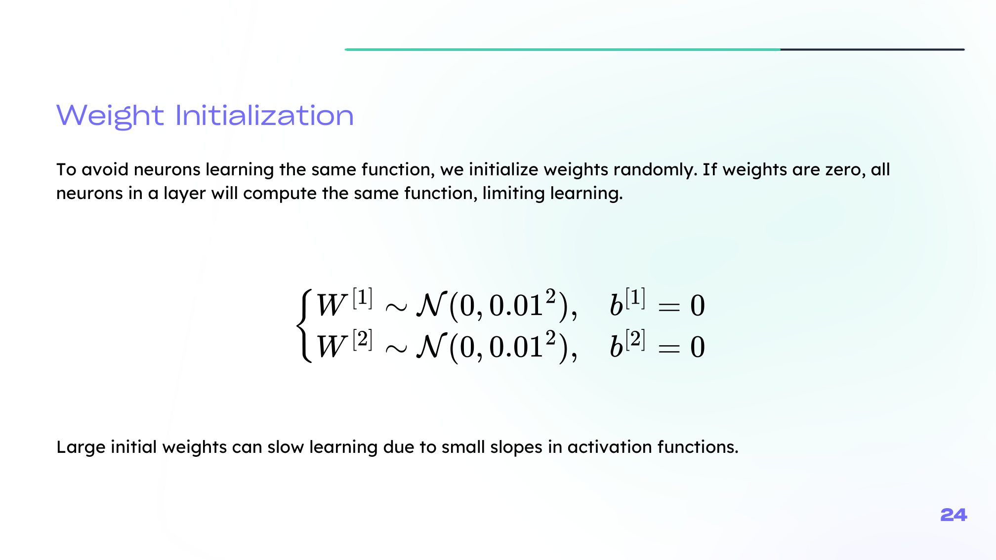
Training deep networks is sensitive to how weights are initialized.
If all weights start at zero:
- neurons in the same layer learn the same function,
- symmetry is never broken,
- learning becomes ineffective.
If weights start too large:
- activations can saturate,
- gradients can vanish or explode,
- optimization becomes unstable.
Your lecture highlights variance-preserving initialization, especially the Xavier-style idea of keeping activations and gradients on a reasonable scale across layers.
For example, Xavier-style initialization uses a variance of roughly
\[ \mathrm{Var}(W) \approx \frac{2}{n_{\mathrm{in}} + n_{\mathrm{out}}}, \]while He initialization for ReLU networks is often written as
\[ \mathrm{Var}(W) \approx \frac{2}{n_{\mathrm{in}}}. \]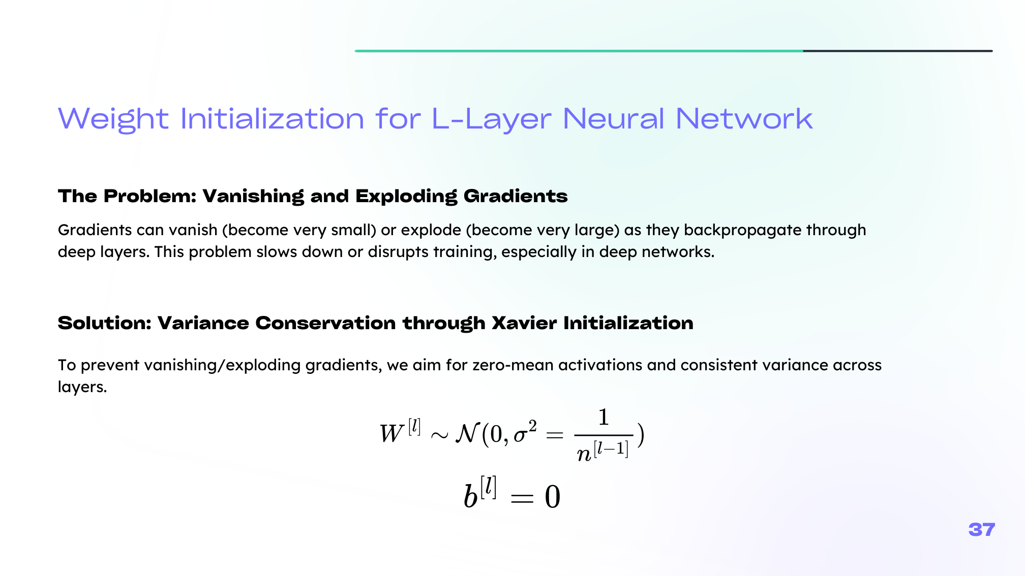
SGD and Mini-Batches
Instead of always computing gradients on the full dataset, we often use smaller subsets.
- Batch gradient descent: stable but expensive
- Stochastic gradient descent (SGD): updates after one example, fast but noisy
- Mini-batch gradient descent: practical compromise used most often
An epoch is one full pass through the training data. The batch size controls how many examples are used per update.
For a mini-batch \(B\), the parameter update takes the familiar form
\[ \theta \leftarrow \theta - \alpha \nabla_\theta J_B(\theta). \]Modern Optimizers
The lecture also reviews several optimizer families:
- Momentum: smooths updates using an exponentially weighted average of past gradients
- AdaGrad: adapts the learning rate per parameter, often useful for sparse settings
- RMSprop: fixes AdaGrad's overly aggressive decay by using a moving average of squared gradients
- Adam: combines momentum and adaptive scaling, which is why it is so widely used
In practice, Adam is a strong default, but SGD with momentum is still common when we want tighter control over generalization.
Momentum itself can be summarized as
\[ v_t = \beta v_{t-1} + (1-\beta)\nabla_\theta J(\theta_t), \qquad \theta_{t+1} = \theta_t - \alpha v_t. \]Hyperparameters and Bias-Variance
Neural networks are highly sensitive to hyperparameters such as:
- learning rate,
- number of layers,
- number of neurons per layer,
- batch size,
- number of epochs,
- activation choice,
- initialization method.
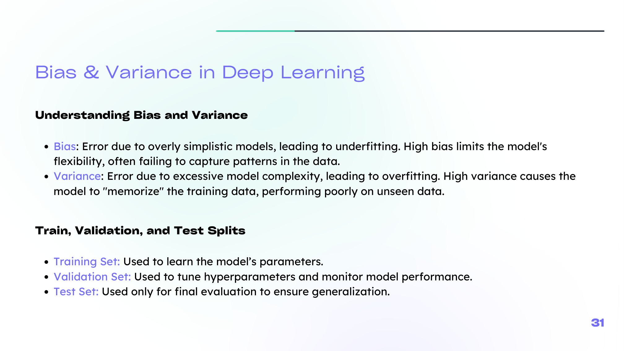
The same logic as in classical ML still applies:
- high bias means the model is too weak or undertrained,
- high variance means the model is too flexible or insufficiently regularized.
Summary
In this lesson we covered:
- What an L-layer network means in practice
- Why initialization is critical in deep models
- The difference between batch, stochastic, and mini-batch gradient descent
- The intuition behind Momentum, AdaGrad, RMSprop, and Adam
- The main hyperparameters that shape training
- Why bias and variance still guide model diagnosis in deep learning
Next: We will study the regularization tools that keep deep models stable and generalizable.