Density-Based Clustering and Practical Guidance
DBSCAN
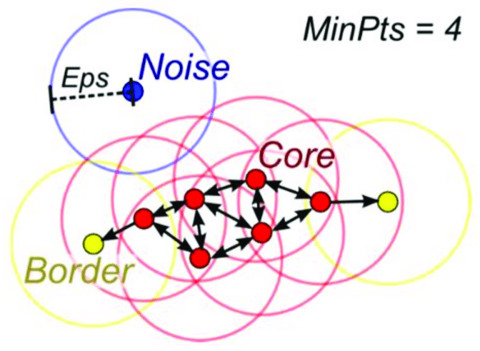
DBSCAN defines clusters as regions of high density separated by sparse regions. Instead of fixing the number of clusters, it uses two parameters:
- \(\varepsilon\): neighborhood radius
- minPts: minimum number of points required to form a dense region
Key ideas:
- a core point has enough neighbors inside its \(\varepsilon\)-neighborhood,
- a border point is close to a core point but not dense enough to expand a cluster,
- a noise point is not density-reachable from any core point.
This is one of DBSCAN's biggest strengths: it can find irregular shapes and mark outliers explicitly.
OPTICS
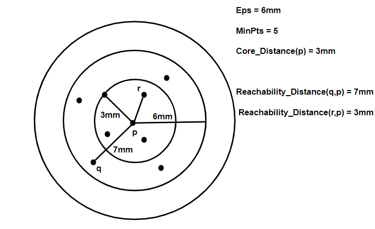
OPTICS extends the same density-based intuition but avoids committing to one fixed density threshold.
Instead of returning just one clustering, it creates:
- an ordering of the points,
- and a reachability distance for each point.
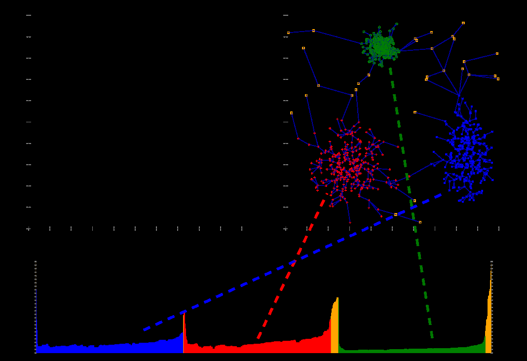
Those outputs are visualized with a reachability plot, where valleys indicate cluster structure.
OPTICS is especially useful when density varies across the dataset and a single global \(\varepsilon\) would be too restrictive.
Practical Guidance
Before clustering, a few habits make a big difference:
- Scale features when distance is sensitive to units.
- Reduce dimension when the original space is very high-dimensional.
- Try more than one method when cluster shape is unclear.
- Inspect stability instead of trusting one run blindly.
Cluster quality can be assessed with:
- silhouette score,
- Calinski-Harabasz or other internal indices,
- and external labels when some benchmark information exists.
Which Method Should You Reach For?
As a quick rule of thumb:
- use hierarchical clustering for exploration and dendrograms,
- use K-means for fast large-scale partitioning,
- use GMMs for soft membership and elliptical clusters,
- use DBSCAN for arbitrary shapes and noise detection,
- use OPTICS when density varies across the data.
Summary
In this lesson we covered:
- How DBSCAN builds clusters from dense neighborhoods
- The roles of core, border, and noise points
- Why OPTICS is useful when density changes across the data
- The importance of scaling, dimension reduction, and stability checks
- How to think about cluster quality in an unsupervised setting
- A practical way to match method choice to problem structure
This completes the current machine learning module. At this point you have a coherent path through linear models, decision trees, evaluation workflows, and clustering.