Simple Linear Regression
What is Linear Regression?
Linear regression is a prediction model that establishes a linear relationship between a target variable and a set of explanatory variables.
The case of one explanatory variable is called simple linear regression:
\[ \hat{Y} = aX + b \]The Gauss–Markov Theorem
The Gauss–Markov theorem states that the ordinary least squares (OLS) estimator has the lowest sampling variance within the class of linear unbiased estimators, if the errors in the linear regression model are:
- Uncorrelated
- Have equal variances (homoscedasticity)
- Have expectation value of zero
The full model with error term:
\[ Y = aX + b + \varepsilon \]where \(\varepsilon\) represents the random error.
Ordinary Least Squares (OLS)
Objective Function
We need to minimize the sum of squared residuals:
\[ \sum_{i=1}^{n} (Y_i - \hat{Y}_i)^2 = \sum_{i=1}^{n} (Y_i - (aX_i + b))^2 \]Solution
By setting the partial derivatives to zero, we find:
\[ \hat{a} = \frac{\text{Cov}(X,Y)}{\text{Var}(X)} = \frac{\sum_{i=1}^{n}(X_i - \bar{X})(Y_i - \bar{Y})}{\sum_{i=1}^{n}(X_i - \bar{X})^2} \]\[ \hat{b} = \bar{Y} - \hat{a}\,\bar{X} \]where:
- \(\bar{X}\) and \(\bar{Y}\) are the sample means
- \(\text{Cov}(X,Y)\) is the covariance between \(X\) and \(Y\)
- \(\text{Var}(X)\) is the variance of \(X\)
Covariance and Correlation
Empirical Covariance
The empirical covariance is defined as:
\[ \text{Cov}(X,Y) = \frac{1}{n-1}\sum_{i=1}^{n}(X_i - \bar{X})(Y_i - \bar{Y}) \]Covariance signifies the direction of the linear relationship between two variables:
- Positive covariance: variables tend to move in the same direction
- Negative covariance: variables tend to move in opposite directions
- Note: \(\text{Cov}(X,X) = \text{Var}(X)\)
Correlation
Correlation refers to the scaled form of covariance:
\[ \text{Cor}(X,Y) = \frac{\text{Cov}(X,Y)}{s_X \cdot s_Y} \]where \(s_X\) and \(s_Y\) are the standard deviations of \(X\) and \(Y\).
Properties:
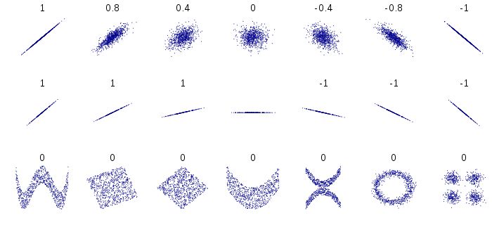
- Correlation is dimensionless and ranges from \(-1\) to \(+1\)
- \(|\text{Cor}(X,Y)| = 1\) indicates a perfect linear relationship
- \(\text{Cor}(X,Y) = 0\) indicates no linear relationship
Errors and Residuals
Statistical Error (Disturbance)
A statistical error \(\varepsilon_i\) is the amount by which an observation differs from its expected value:
\[ Y_i = aX_i + b + \varepsilon_i \quad \Rightarrow \quad \varepsilon_i = Y_i - (aX_i + b) \]Residual
A residual \(r_i\) is the observable estimate of the unobservable statistical error:
\[ r_i = \hat{\varepsilon}_i = Y_i - (\hat{a}X_i + \hat{b}) = Y_i - \hat{Y}_i \]Key difference:
- Errors \(\varepsilon_i\) involve the true (unknown) parameters \(a\) and \(b\)
- Residuals \(r_i\) involve the estimated parameters \(\hat{a}\) and \(\hat{b}\)
Visualizing OLS Fit
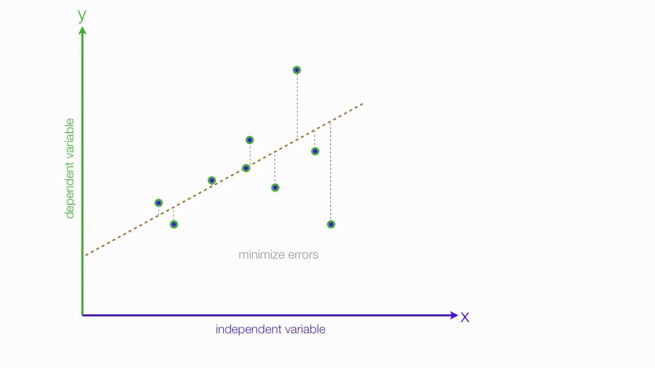
The regression line minimizes the sum of squared vertical distances (residuals) from each point to the line.
Summary
In this lesson we covered:
- ✅ The definition of simple linear regression
- ✅ The Gauss–Markov theorem and OLS properties
- ✅ How to derive coefficient estimates using calculus
- ✅ The relationship between covariance and correlation
- ✅ The distinction between errors and residuals
Next: We'll explore how to assess the quality of our fit, test hypotheses about coefficients, and diagnose potential problems through residual analysis.