Inference & Diagnostic
Residual Analysis
Residual analysis is critical for validating our regression assumptions and identifying potential problems.
Types of Residual Plots
1. Residuals vs Fitted Values
A plot of residuals against fitted values should show no pattern. If a pattern is observed, there may be issues:
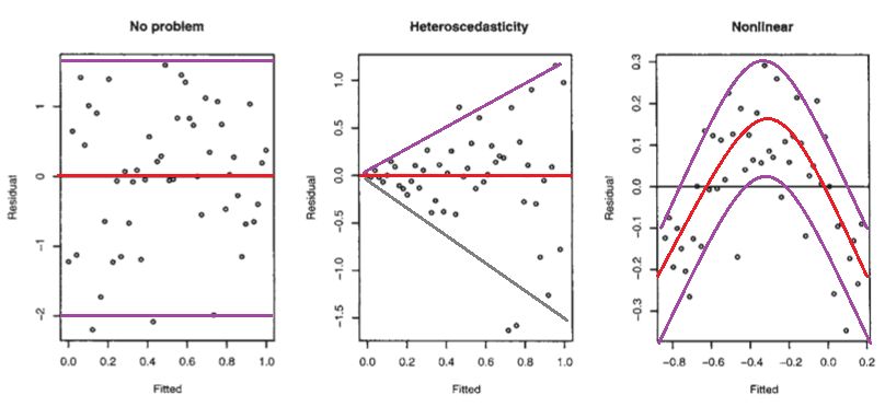
- No problem: Random scatter around zero
- Heteroscedasticity: Variance increases with fitted values
- Nonlinear: Curved pattern suggests missing nonlinear terms
Key Insights from Residual Plots
-
Heteroscedasticity: The variance of residuals is not constant → violates Gauss–Markov assumptions
- Solution: Transform the target variable (logarithm, square root)
-
Nonlinearity: Scatterplots of residuals vs predictors show patterns
- Solution: Add polynomial terms or other transformations
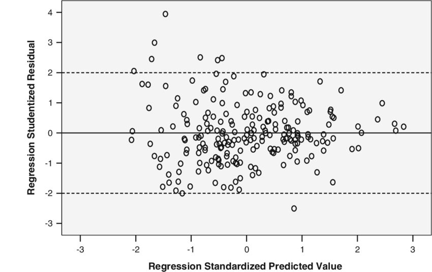
Studentized Residuals
To identify outliers, we standardize residuals. Under the assumption of normality of errors:
\[ t_i = \frac{\hat{\varepsilon}_i}{\hat{\sigma}\sqrt{1 - h_{ii}}} \]where:
-
\(\hat{\sigma}\) is the estimated standard deviation of residuals:
\[ \hat{\sigma} = \sqrt{\frac{1}{n-2}\sum_{j=1}^{n}\hat{\varepsilon}_j^2} \] -
\(h_{ii}\) is the leverage (diagonal element of the hat matrix):
\[ h_{ii} = \frac{1}{n} + \frac{(X_i - \bar{X})^2}{\sum_{j=1}^{n}(X_j - \bar{X})^2} \]
Under the null hypothesis, \(t_i\) follows a Student's t-distribution with \(n-2\) degrees of freedom.
Outlier Detection
Studentized residuals help identify observations that don't fit the model:
- Points with \(|t_i| > 2\) or \(|t_i| > 3\) are potential outliers
-
Target Transformation
When to transform? Target transformation is necessary to cope with heteroscedasticity, which is often linked to the skewness of the target distribution.
Common Transformations
| Problem | Transformation | Effect |
|---|---|---|
| Right-skewed target | \(\log(Y)\) | Reduces skewness, stabilizes variance |
| Variance increases with Y | \(\sqrt{Y}\) | Moderate stabilization |
| Count data | \(\log(Y+1)\) | Handles zeros |
Example: Housing prices are often right-skewed. After log transformation, the distribution becomes more symmetric and residual variance is more constant.
Diagnostic Plots
Modern statistical software provides multiple diagnostic plots. Here's what each reveals:
1. Residuals vs Fitted
Purpose: Detect non-linearity and heteroscedasticity Ideal: Random scatter with no pattern
2. Normal Q-Q Plot
Purpose: Check normality of residuals Ideal: Points lie on the diagonal line
If residuals deviate from the line:
- Heavy tails: Points curve away at extremes
- Skewness: Systematic deviation on one side
3. Scale-Location Plot
Purpose: Check homoscedasticity (equal variance) Ideal: Horizontal line with evenly spread points
4. Residuals vs Leverage
Purpose: Identify influential observations Uses: Cook's distance
Influential Observations
Cook's Distance
Cook's distance \(D_i\) measures how much the regression coefficients change when observation \(i\) is removed:
\[ D_i = \frac{\sum_{j=1}^{n}(\hat{y}_j - \hat{y}_{j(i)})^2}{p\hat{\sigma}^2} \]where \(\hat{y}_{j(i)}\) is the fitted value when observation \(i\) is excluded.
Rule of thumb:
- \(D_i > 0.5\): Potentially influential
- \(D_i > 1\): Highly influential
DFFITS
DFFITS (Difference in Fits) is a scaled measure of change in the predicted value:
\[ \text{DFFITS}_i = t_i \sqrt{\frac{h_{ii}}{1 - h_{ii}}} \]Cutoff (Belsley, Kuh, and Welsch):
\[ 2\sqrt{\frac{p}{n}} \]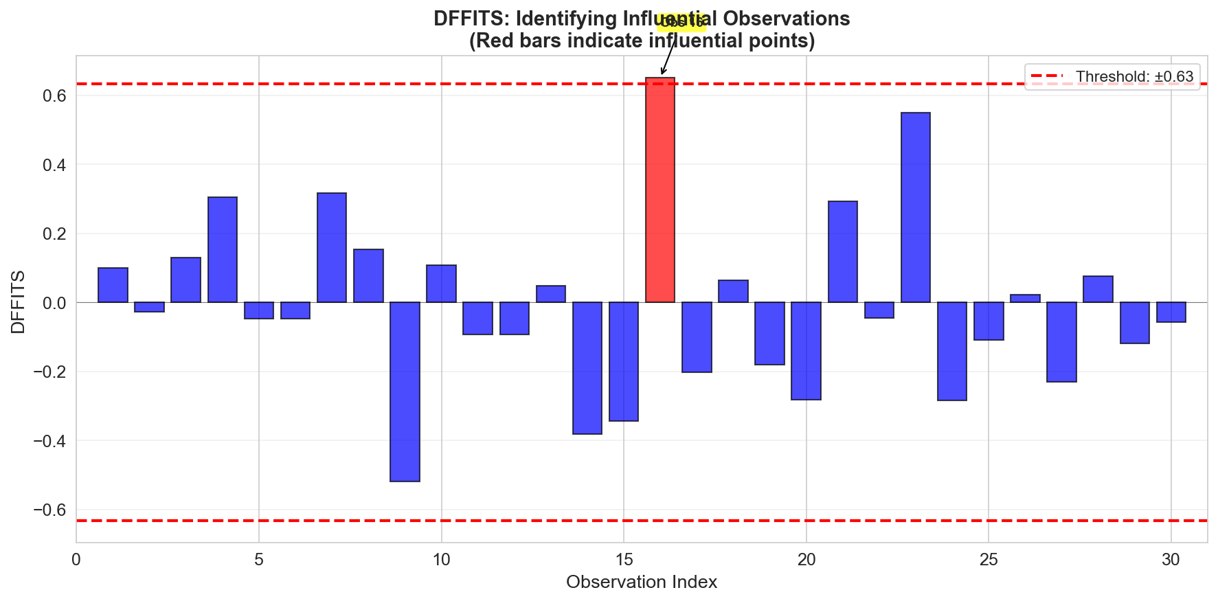
Coefficient of Determination (R²)
\(R^2\) measures the proportion of variance in \(Y\) explained by \(X\):
\[ R^2 = \frac{\text{SSR}}{\text{SST}} = 1 - \frac{\text{SSE}}{\text{SST}} = 1 - \frac{\sum(Y_i - \hat{Y}_i)^2}{\sum(Y_i - \bar{Y})^2} \]where:
- SST (Total Sum of Squares) = \(\sum(Y_i - \bar{Y})^2\)
- SSR (Regression Sum of Squares) = \(\sum(\hat{Y}_i - \bar{Y})^2\)
- SSE (Error Sum of Squares) = \(\sum(Y_i - \hat{Y}_i)^2\)
Interpretation:
- \(R^2 = 0\): Model explains no variance (no better than the mean)
- \(R^2 = 1\): Perfect fit (all variance explained)
- For simple linear regression: \(R^2 = \text{Cor}(Y, \hat{Y})^2\)
Summary
In this lesson we covered:
- ✅ Residual analysis to detect violations of assumptions
- ✅ Studentized residuals for outlier detection
- ✅ Target transformations to handle heteroscedasticity
- ✅ Diagnostic plots (Q-Q, scale-location, leverage)
- ✅ Influential observations (Cook's distance, DFFITS)
- ✅ R² as a measure of model fit
Next: We'll extend to multiple regression with several predictors, learning matrix notation and the normal equation.