Model Selection and Regularization
Inference in Regression
Under the assumption of normality of the errors \(\varepsilon_i \sim \mathcal{N}(0, \sigma^2)\), we can perform statistical inference about the coefficients.
Distribution of Coefficient Estimators
From the normal equation \(\hat{a} = (X^T X)^{-1} X^T Y\), we have:
\[ E(\hat{a}) = a \]\[ \text{VAR}(\hat{a}) = \sigma^2 (X^T X)^{-1} \]Therefore:
\[ \hat{a} \sim \mathcal{N}(a, \sigma^2 (X^T X)^{-1}) \]Estimating the Error Variance
The variance of the residuals can be approximated using the residual sum of squares:
\[ \hat{\sigma}^2 = \frac{\sum_{i=1}^{n} (\hat{\varepsilon}_i)^2}{n - p} = \frac{\|e\|^2}{n - p} \]where \(p\) is the number of parameters (including intercept).
Statistical Tests for Coefficients
Hypothesis Test for Individual Coefficients
To test whether a coefficient \(a_j\) is significantly different from zero:
Hypotheses:
- \(H_0\): \(a_j = 0\) (coefficient has no effect)
- \(H_1\): \(a_j \neq 0\) (coefficient is significant)
Test statistic:
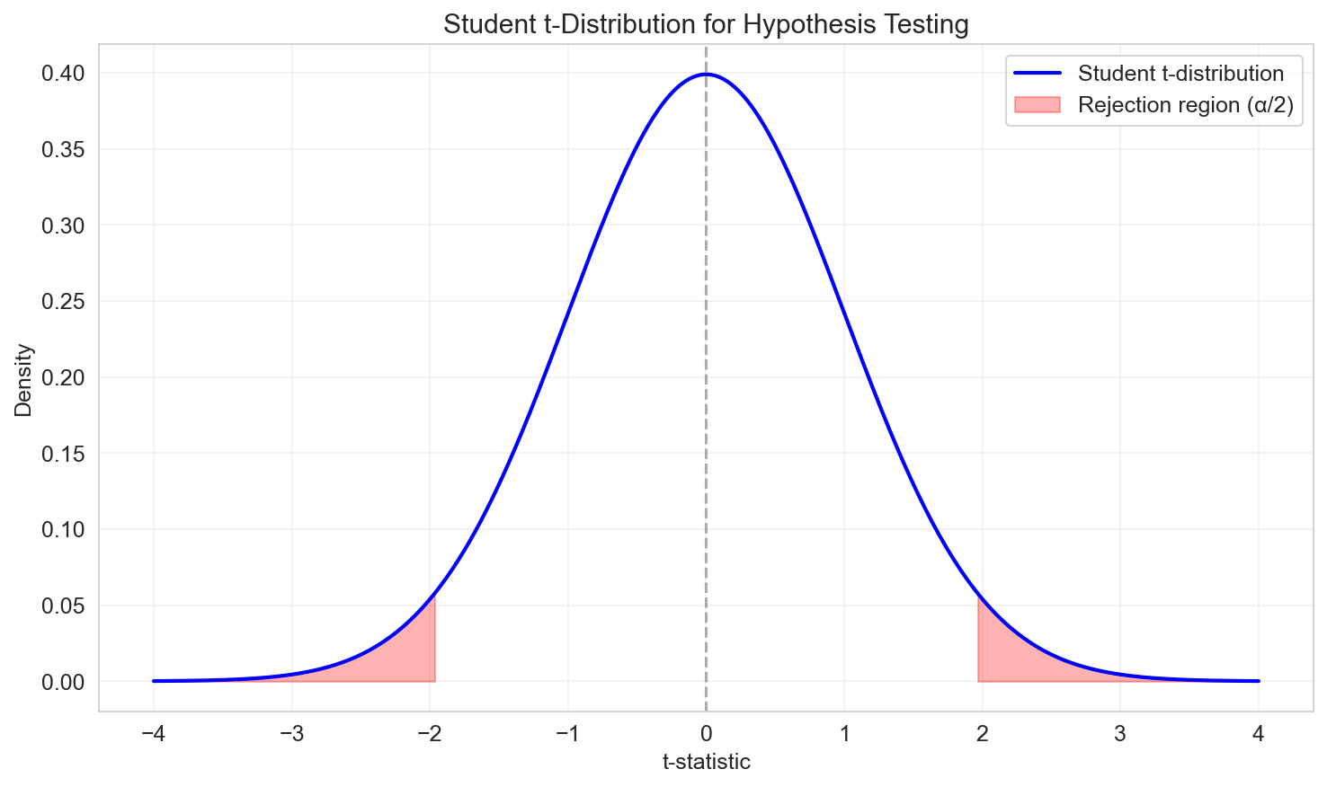
Under \(H_0\), the t-statistic follows a Student's t-distribution with \(n - p\) degrees of freedom:
\[ t_j = \frac{\hat{a}_j}{s_{\hat{a}_j}} \sim t_{n-p} \]where \(s_{\hat{a}_j}\) is the standard error of \(\hat{a}_j\), obtained from the diagonal of:
\[ \text{VAR}(\hat{a}) = \hat{\sigma}^2 (X^T X)^{-1} \]Decision rule:
- If \(|t_j| > t_{\alpha/2, n-p}\), reject \(H_0\) at significance level \(\alpha\)
- Typically use \(\alpha = 0.05\) (5%) or \(\alpha = 0.01\) (1%)
Confidence Intervals
Confidence Interval for Coefficients
Based on the distribution of \(\hat{a}_j\), a \((1-\alpha)\) confidence interval for \(a_j\) is:
\[ \hat{a}_j \in \left[ \hat{a}_j - s_{\hat{a}_j} \, t_{\alpha/2, n-p} \;,\; \hat{a}_j + s_{\hat{a}_j} \, t_{\alpha/2, n-p} \right] \]where \(t_{\alpha/2, n-p}\) is the critical value from the Student's t-distribution.
Interpretation: We are \((1-\alpha) \times 100\%\) confident that the true parameter \(a_j\) lies within this interval.
Confidence Interval for Predictions
For a new observation with predictors \(x_{\text{new}}\), the predicted value is:
\[ \hat{y}_{\text{new}} = x_{\text{new}}^T \hat{a} \]The variance of the prediction is:
\[ \text{VAR}(\hat{y}_{\text{new}}) = \sigma^2 x_{\text{new}}^T (X^T X)^{-1} x_{\text{new}} \]A \((1-\alpha)\) confidence interval for the prediction is:
\[ \hat{y}_{\text{new}} \in \left[ \hat{y}_{\text{new}} - s_{\hat{y}} \, t_{\alpha/2, n-p} \;,\; \hat{y}_{\text{new}} + s_{\hat{y}} \, t_{\alpha/2, n-p} \right] \]where:
\[ s_{\hat{y}} = \hat{\sigma} \sqrt{x_{\text{new}}^T (X^T X)^{-1} x_{\text{new}}} \]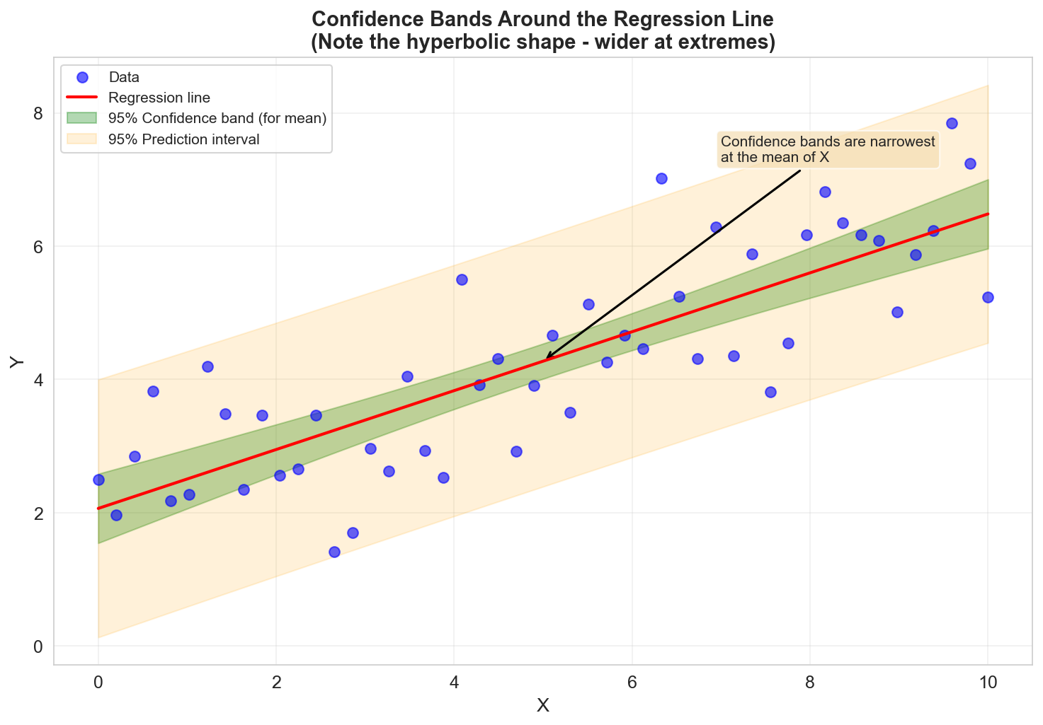
Note: In simple linear regression, confidence bands have a hyperbolic shape, wider at the extremes of the data range.
Adjusted R²
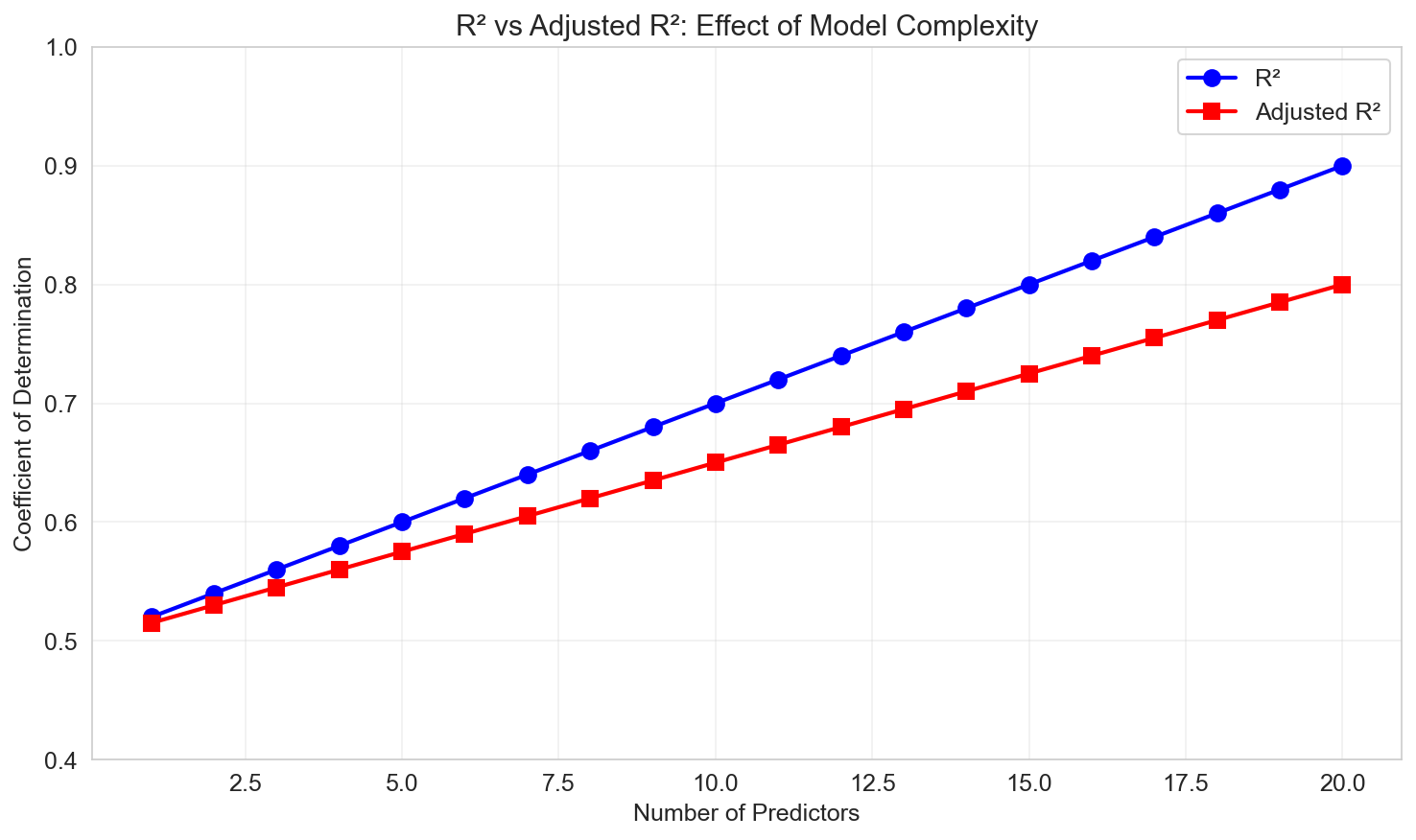
The Problem with R²
\(R^2\) is at least weakly increasing with the number of regressors:
\[ R^2 = 1 - \frac{\text{SSE}}{\text{SST}} \]Adding more predictors (even irrelevant ones) can never decrease \(R^2\). This makes it unsuitable for comparing models with different numbers of variables.
Adjusted R²
The adjusted R² penalizes model complexity:
\[ \bar{R}^2 = 1 - \frac{\text{SSE}/(n-p)}{\text{SST}/(n-1)} = 1 - (1 - R^2) \frac{n-1}{n-p} \]Properties:
- Can decrease if adding a predictor doesn't improve fit enough to justify the extra parameter
- More appropriate for model comparison
- Still has limitations (not a likelihood-based criterion)
The F-Distribution
The F-distribution with parameters \(d_1\) and \(d_2\) arises as the ratio of two independent chi-squared variables:
If \(S_1 \sim \chi^2_{d_1}\) and \(S_2 \sim \chi^2_{d_2}\), then:
\[ F = \frac{S_1 / d_1}{S_2 / d_2} \sim F(d_1, d_2) \]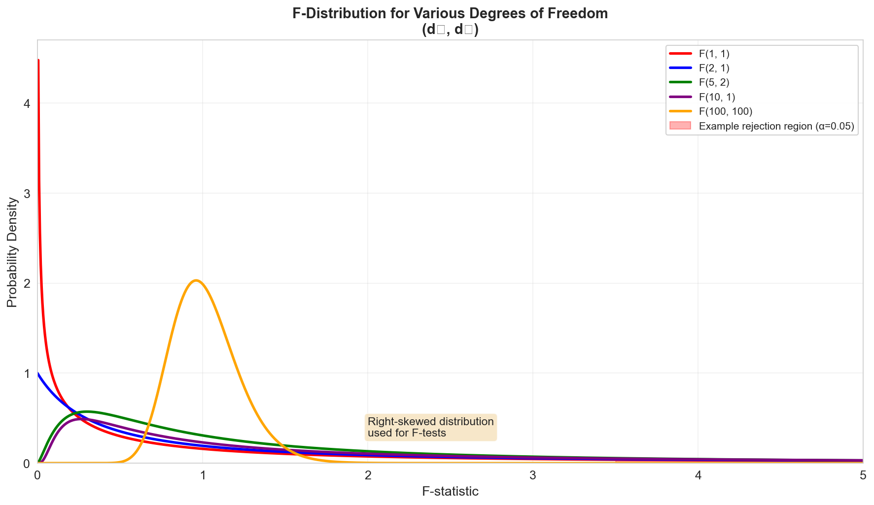
Properties:
- Always non-negative
- Right-skewed
- Shape depends on both \(d_1\) and \(d_2\)
The F-Test for Regression
Overall Significance Test (Simple Regression)
The F-test of overall significance compares a model with predictors to an intercept-only model.
Hypotheses:
- \(H_0\): \(a = 0\) (the model is no better than the mean)
- \(H_1\): \(a \neq 0\) (the model has explanatory power)
Test statistic:
\[ F_{\text{obs}} = \frac{\text{MSR}}{\text{MSE}} = \frac{\text{SSR}/1}{\text{SSE}/(n-2)} \]where:
- SSR (Sum of Squares Regression) = \(\sum_{i=1}^{n} (\hat{Y}_i - \bar{Y})^2\)
- SSE (Sum of Squares Error) = \(\sum_{i=1}^{n} (Y_i - \hat{Y}_i)^2\)
- MSR (Mean Square Regression) = \(\text{SSR} / 1\)
- MSE (Mean Square Error) = \(\text{SSE} / (n-2)\)
Under \(H_0\):
\[ F_{\text{obs}} \sim F(1, n-2) \]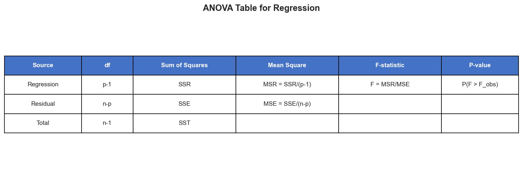
Relationship to R²
For simple linear regression, there's a direct relationship:
\[ F_{\text{obs}} = \frac{R^2}{1 - R^2} \cdot (n - 2) \]F-Test for Nested Models
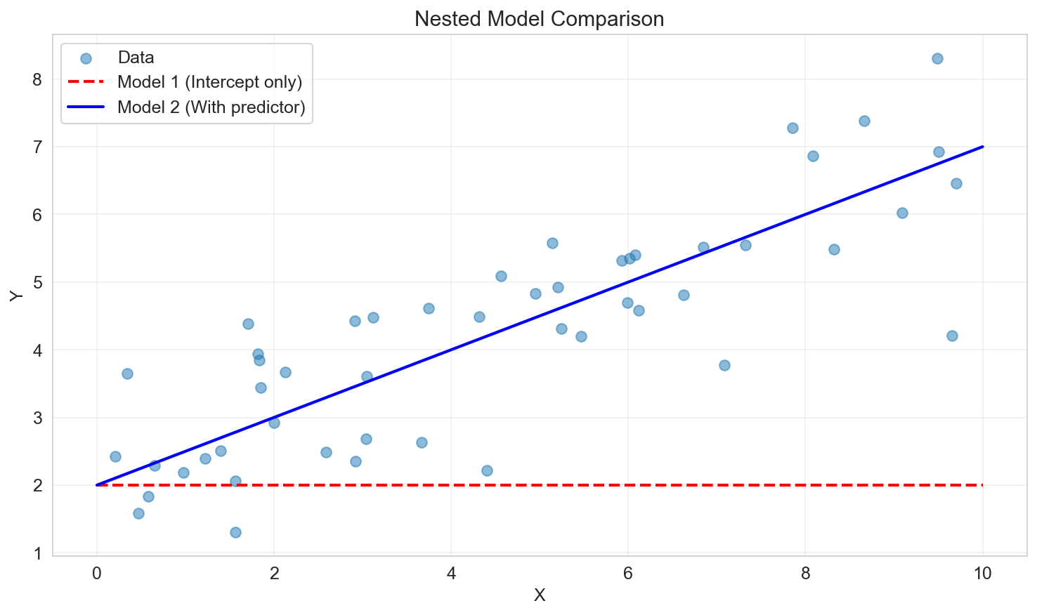
Comparing Two Models
Consider two nested models:
- Model 1 (restricted): \(p_1\) parameters
- Model 2 (unrestricted): \(p_2\) parameters, where \(p_2 > p_1\)
Model 1 is "nested" within Model 2 if every model in 1 can be represented by some choice of parameters in 2.
Hypotheses:
- \(H_0\): Model 2 does not provide a significantly better fit than Model 1
- \(H_1\): Model 2 provides a significantly better fit
Test statistic:
\[ F = \frac{(\text{SSE}_1 - \text{SSE}_2) / (p_2 - p_1)}{\text{SSE}_2 / (n - p_2)} \sim F(p_2 - p_1, n - p_2) \]Interpretation:
- Large \(F\) → Reject \(H_0\) → The additional predictors improve the model
- Small \(F\) → Fail to reject \(H_0\) → The additional predictors are not justified
Model Selection Methods
When we have many potential predictors, we need systematic methods to select which ones to include.
1. Backward Elimination
Algorithm:
- Start with the full model (all predictors)
- Choose a significance level to stay (SLS), e.g., 0.05
- Fit the model and find the predictor with the largest p-value
- If \(p\text{-value} > \text{SLS}\), remove that predictor
- Refit the model with remaining predictors
- Repeat steps 3-5 until all predictors have \(p\text{-value} \leq \text{SLS}\)
Pros: Simple, considers interactions among predictors Cons: Can miss important variables if they're only significant in combination with others
2. Forward Selection
Algorithm:
- Start with the intercept-only model (no predictors)
- Choose a significance level to enter (SLE), e.g., 0.05
- Fit all simple models (one predictor each)
- Find the predictor with the smallest p-value
- If \(p\text{-value} < \text{SLE}\), add that predictor
- Among remaining predictors, fit two-variable models including the selected variable
- Repeat steps 4-6 until no additional variables have \(p\text{-value} < \text{SLE}\)
Pros: Computationally efficient for large predictor sets Cons: Once a variable is added, it stays (can't remove it later)
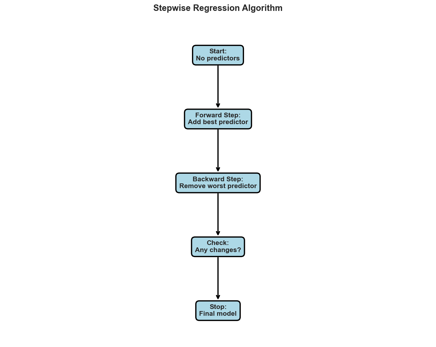
3. Stepwise Regression
Algorithm: Combines forward selection and backward elimination:
- Start like forward selection
- After each new variable is added, perform backward elimination on all variables
- Continue until no variables can be added or removed
Pros: More flexible than forward or backward alone Cons: Still greedy, no guarantee of finding the optimal model
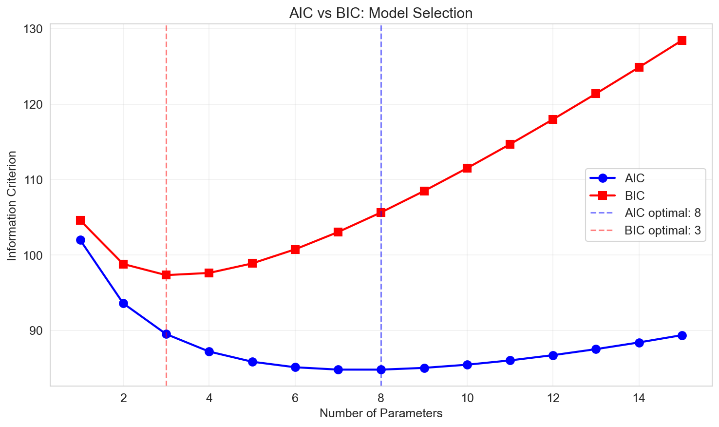
Information Criteria
Akaike Information Criterion (AIC)
\[ \text{AIC} = 2p - 2\ln(L) \]where:
- \(p\) is the number of parameters
- \(L\) is the maximized likelihood
For linear regression:
\[ \text{AIC} = n \ln\left(\frac{\text{SSE}}{n}\right) + 2p \]Lower AIC is better (balances fit and complexity)
Bayesian Information Criterion (BIC)
\[ \text{BIC} = p \ln(n) - 2\ln(L) \]For linear regression:
\[ \text{BIC} = n \ln\left(\frac{\text{SSE}}{n}\right) + p \ln(n) \]Lower BIC is better
BIC vs AIC:
- BIC penalizes complexity more heavily than AIC (especially for large \(n\))
- BIC tends to select simpler models than AIC
- Both are useful; often compare multiple criteria
Dealing with Collinearity
What is Collinearity?
Collinearity occurs when predictors are highly correlated with each other.
Perfect collinearity: One predictor is an exact linear combination of others
- \(X^T X\) is singular (not invertible)
- Parameters are non-identifiable
High collinearity (but not perfect):
- \(X^T X\) is technically invertible but numerically unstable
- Coefficient estimates have large standard errors
- Small changes in data cause large changes in coefficients
Detecting Collinearity
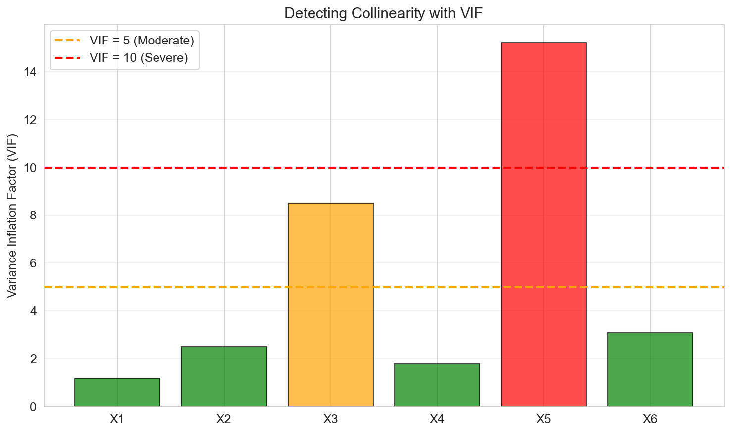
Variance Inflation Factor (VIF):
For predictor \(j\):
\[ \text{VIF}_j = \frac{1}{1 - R_j^2} \]where \(R_j^2\) is the \(R^2\) from regressing \(X_j\) on all other predictors.
Rule of thumb:
- \(\text{VIF} > 5\): Moderate collinearity
- \(\text{VIF} > 10\): Severe collinearity
Solutions to Collinearity
- Remove one of the correlated predictors
- Combine predictors (e.g., create an average or principal component)
- Regularization methods: Ridge, Lasso, Elastic Net
- Collect more data (if possible)
Regularization: Ridge and Lasso
When \(p\) is large or predictors are highly correlated, regularization can help.
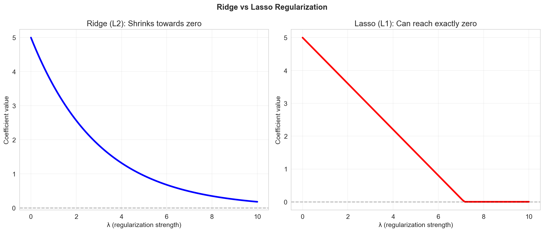
Ridge Regression
Objective:
\[ \min_a \left\{ \|Y - Xa\|^2 + \lambda \|a\|^2 \right\} \]- Adds an \(\ell_2\) penalty on coefficient magnitudes
- Shrinks coefficients toward zero (but never exactly zero)
- Solution: \(\hat{a}_{\text{ridge}} = (X^T X + \lambda I)^{-1} X^T Y\)
Lasso Regression
Objective:
\[ \min_a \left\{ \|Y - Xa\|^2 + \lambda \|a\|_1 \right\} \]- Adds an \(\ell_1\) penalty on coefficient magnitudes
- Can set some coefficients exactly to zero (variable selection)
- No closed-form solution (requires optimization algorithms)
Choosing \(\lambda\): Use cross-validation to select the regularization parameter that minimizes prediction error on held-out data.
Summary
In this lesson we covered:
- ✅ Inference in regression: hypothesis tests and confidence intervals for coefficients
- ✅ Adjusted R² to account for model complexity
- ✅ F-distribution and F-tests for overall significance and nested model comparison
- ✅ Model selection methods: backward elimination, forward selection, stepwise regression
- ✅ Information criteria: AIC and BIC
- ✅ Collinearity: detection (VIF) and solutions
- ✅ Regularization: Ridge and Lasso for high-dimensional problems
Next: We'll extend beyond normal linear regression to Generalized Linear Models (GLM) and logistic regression for classification problems.