Generalized Linear Models (GLM) and Logistic Regression
Generalized Linear Models (GLM)
The generalized linear model (GLM) is a generalization of ordinary linear regression that allows the response variable to have distributions other than the normal distribution.
The Three Components of a GLM
A GLM consists of three elements:
1. Exponential Family of Probability Distributions
The response variable \(Y\) follows a distribution from the exponential family:
- Normal distribution (ordinary linear regression)
- Bernoulli distribution (logistic regression)
- Poisson distribution (count data)
- Exponential distribution (survival/time-to-event data)
- Gamma distribution (positive continuous data with skewness)
2. Linear Predictor
\[ \eta = Xa = a_0 + a_1 X_1 + a_2 X_2 + \ldots + a_p X_p \]This is the same linear combination of predictors as in ordinary regression.
3. Link Function
A link function \(g\) connects the expected value \(\mu = E(Y)\) to the linear predictor:
\[ g(\mu) = \eta \]or equivalently:
\[ E(Y) = \mu = g^{-1}(\eta) \]GLM Formula
The generalized linear model is defined by:
\[ E(Y) = g^{-1}(Xa) \]For ordinary linear regression:
- Distribution: Normal
- Link function: \(g(x) = x\) (identity link)
- Result: \(E(Y) = Xa\)
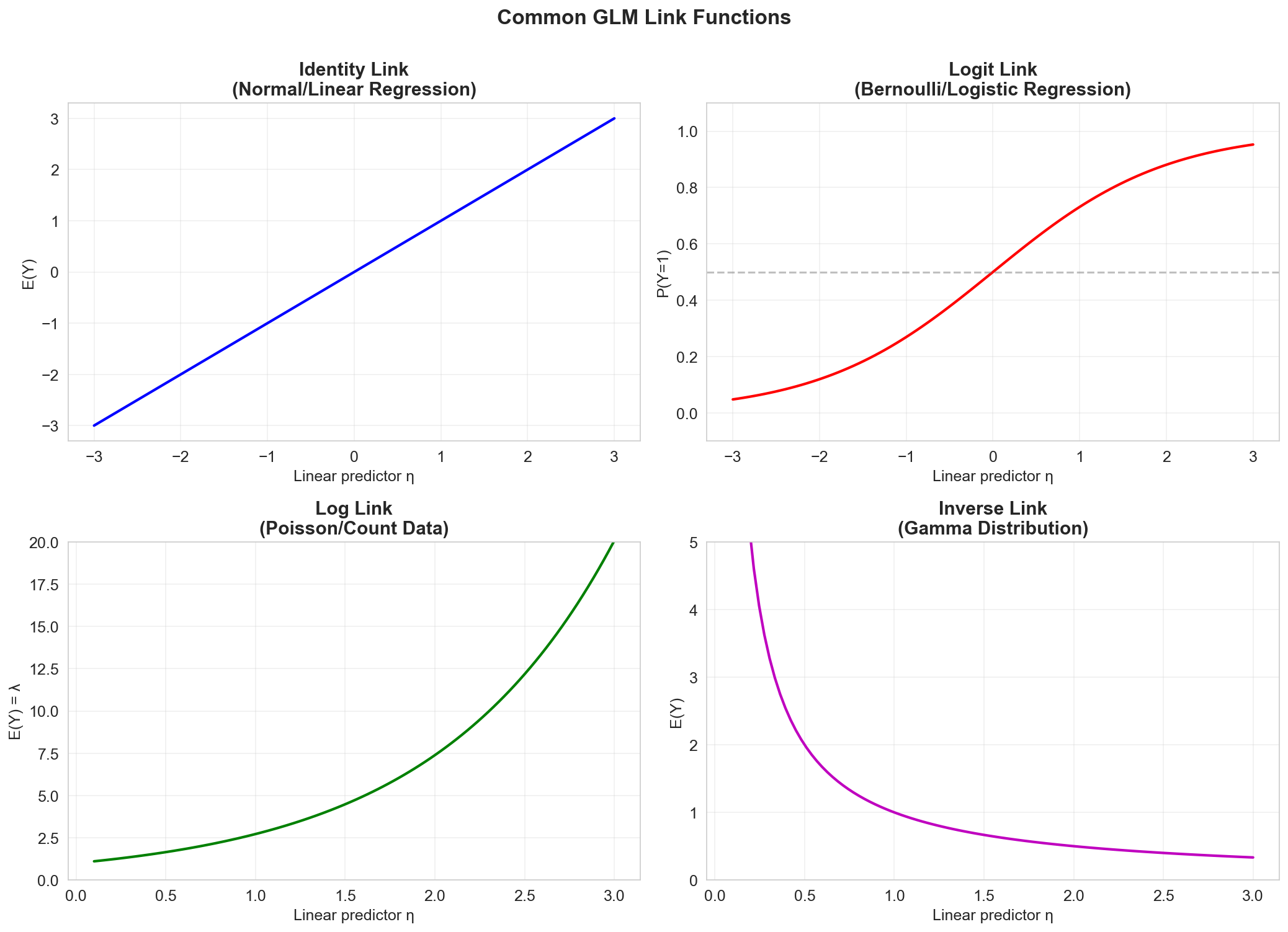
Common Link Functions
Different response distributions have corresponding canonical link functions:
| Distribution | Support | Link Function \(g(\mu)\) | Inverse Link \(g^{-1}(\eta)\) | Use Case |
|---|---|---|---|---|
| Normal | \(\mathbb{R}\) | \(\mu\) (identity) | \(\eta\) | Continuous responses |
| Bernoulli | \(\{0, 1\}\) | \(\log\left(\frac{\mu}{1-\mu}\right)\) (logit) | \(\frac{e^\eta}{1+e^\eta}\) | Binary classification |
| Poisson | \(\mathbb{N}\) | \(\log(\mu)\) | \(e^\eta\) | Count data |
| Gamma | \(\mathbb{R}^+\) | \(\frac{1}{\mu}\) (inverse) | \(\frac{1}{\eta}\) | Positive continuous (e.g., insurance claims) |
Parameter Estimation: Maximum Likelihood
In GLMs, the unknown parameters \(a\) are typically estimated using maximum likelihood estimation (MLE):
\[ \hat{a} = \arg\max_a \, L(a \mid Y, X) = \arg\max_a \sum_{i=1}^{n} \log p(y_i \mid x_i, a) \]Unlike ordinary regression (which has a closed-form solution), GLMs generally require iterative optimization algorithms:
- Newton-Raphson method
- Iteratively Reweighted Least Squares (IRLS)
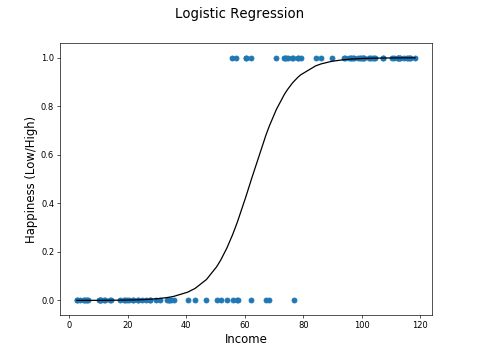
Logistic Regression
Logistic regression is used when the response variable \(Y\) is binary (taking values 0 or 1).
Binary Response Distribution
When \(Y_i \in \{0, 1\}\), we model it as a Bernoulli random variable:
\[ Y_i \sim \text{Bernoulli}(p_i) \]where \(p_i = P(Y_i = 1)\) is the probability of "success" for observation \(i\).
The expected value is:
\[ E(Y_i) = \mu_i = p_i \]The Logit Link Function
The logit (log-odds) link function is the canonical link for logistic regression:
\[ g(\mu) = \log\left(\frac{\mu}{1 - \mu}\right) = \log\left(\frac{p}{1 - p}\right) \]This maps probabilities from \([0, 1]\) to the entire real line \((-\infty, +\infty)\).
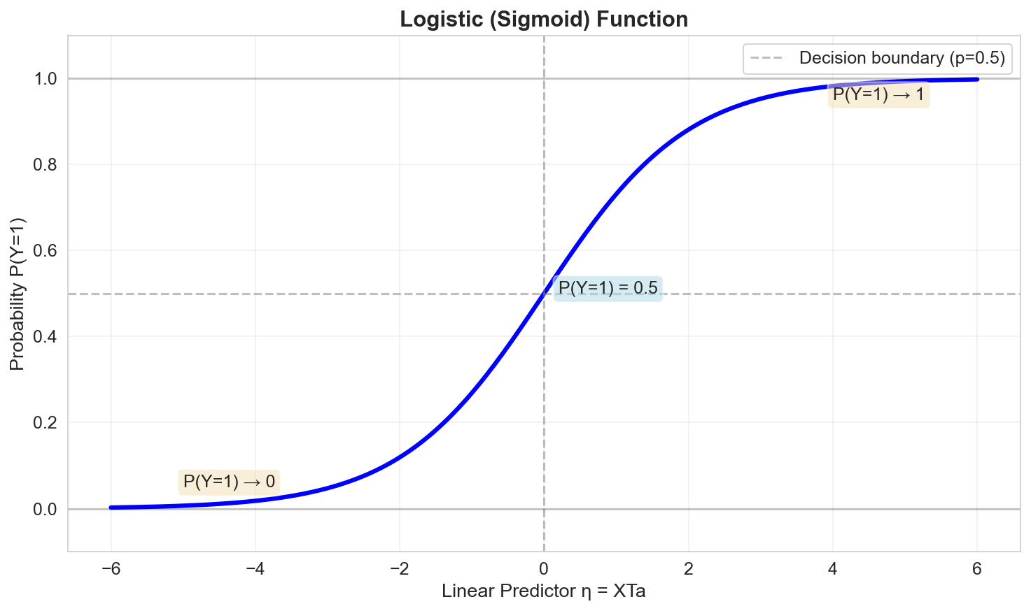
Inverse Link: The Logistic Function
Inverting the logit gives the logistic function (sigmoid):
\[ \mu = g^{-1}(\eta) = \frac{\exp(\eta)}{1 + \exp(\eta)} = \frac{1}{1 + \exp(-\eta)} \]This maps the linear predictor \(\eta\) back to a probability in \([0, 1]\).
Logistic Regression Model
For a binary response, the logistic regression model is:
\[ \log\left(\frac{p_i}{1 - p_i}\right) = a_0 + a_1 X_{i1} + a_2 X_{i2} + \ldots + a_p X_{ip} \]Equivalently:
\[ p_i = P(Y_i = 1 \mid X_i) = \frac{\exp(a_0 + a_1 X_{i1} + \ldots + a_p X_{ip})}{1 + \exp(a_0 + a_1 X_{i1} + \ldots + a_p X_{ip})} \]Interpretation of coefficients:
- \(a_j > 0\): Increasing \(X_j\) increases the log-odds (and thus the probability) of \(Y = 1\)
- \(a_j < 0\): Increasing \(X_j\) decreases the log-odds of \(Y = 1\)
- \(\exp(a_j)\): The odds ratio associated with a one-unit increase in \(X_j\)
Maximum Likelihood for Logistic Regression
Likelihood Function
For binary data, the likelihood is:
\[ L(a) = \prod_{i=1}^{n} p_i^{y_i} (1 - p_i)^{1 - y_i} \]Log-Likelihood
Taking the logarithm:
\[ \ell(a) = \sum_{i=1}^{n} \left[ y_i \log(p_i) + (1 - y_i) \log(1 - p_i) \right] \]Substituting \(p_i = \frac{\exp(\eta_i)}{1 + \exp(\eta_i)}\) where \(\eta_i = x_i^T a\):
\[ \ell(a) = \sum_{i=1}^{n} \left[ y_i \eta_i - \log(1 + \exp(\eta_i)) \right] \]Negative Log-Likelihood (Loss Function)
In practice, we minimize the negative log-likelihood:
\[ \text{NLL}(a) = -\ell(a) = -\sum_{i=1}^{n} \left[ y_i \log(p_i) + (1 - y_i) \log(1 - p_i) \right] \]This is also known as the binary cross-entropy loss.
Optimization: There is no closed-form solution. We use iterative algorithms:
- Gradient descent
- Newton-Raphson
- IRLS (Iteratively Reweighted Least Squares)
Interpretation and Decision Boundary
Odds and Odds Ratio
The odds of \(Y = 1\) are:
\[ \text{Odds} = \frac{p}{1 - p} = \exp(\eta) = \exp(a_0 + a_1 X_1 + \ldots + a_p X_p) \]For a one-unit increase in \(X_j\):
\[ \text{Odds Ratio} = \exp(a_j) \]Example: If \(\exp(a_1) = 2.5\), then a one-unit increase in \(X_1\) multiplies the odds of \(Y = 1\) by 2.5.
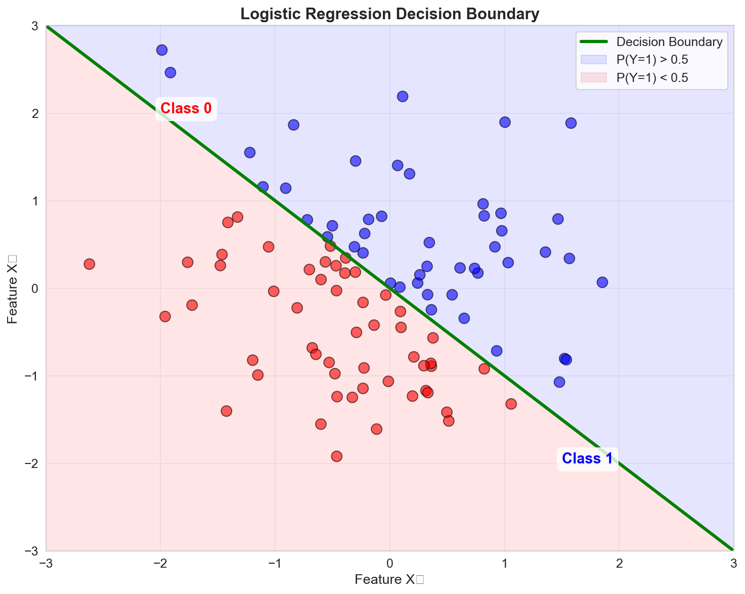
Decision Boundary
To classify a new observation, we typically use a threshold (e.g., \(p = 0.5\)):
\[ \hat{Y} = \begin{cases} 1 & \text{if } p > 0.5 \\ 0 & \text{otherwise} \end{cases} \]The decision boundary is where \(p = 0.5\), which occurs when:
\[ \eta = a_0 + a_1 X_1 + \ldots + a_p X_p = 0 \]For two predictors, this defines a line in the feature space.
Model Evaluation for Logistic Regression
Deviance
The deviance is a measure of model fit:
\[ D = -2 \ell(a) \]Lower deviance indicates better fit.
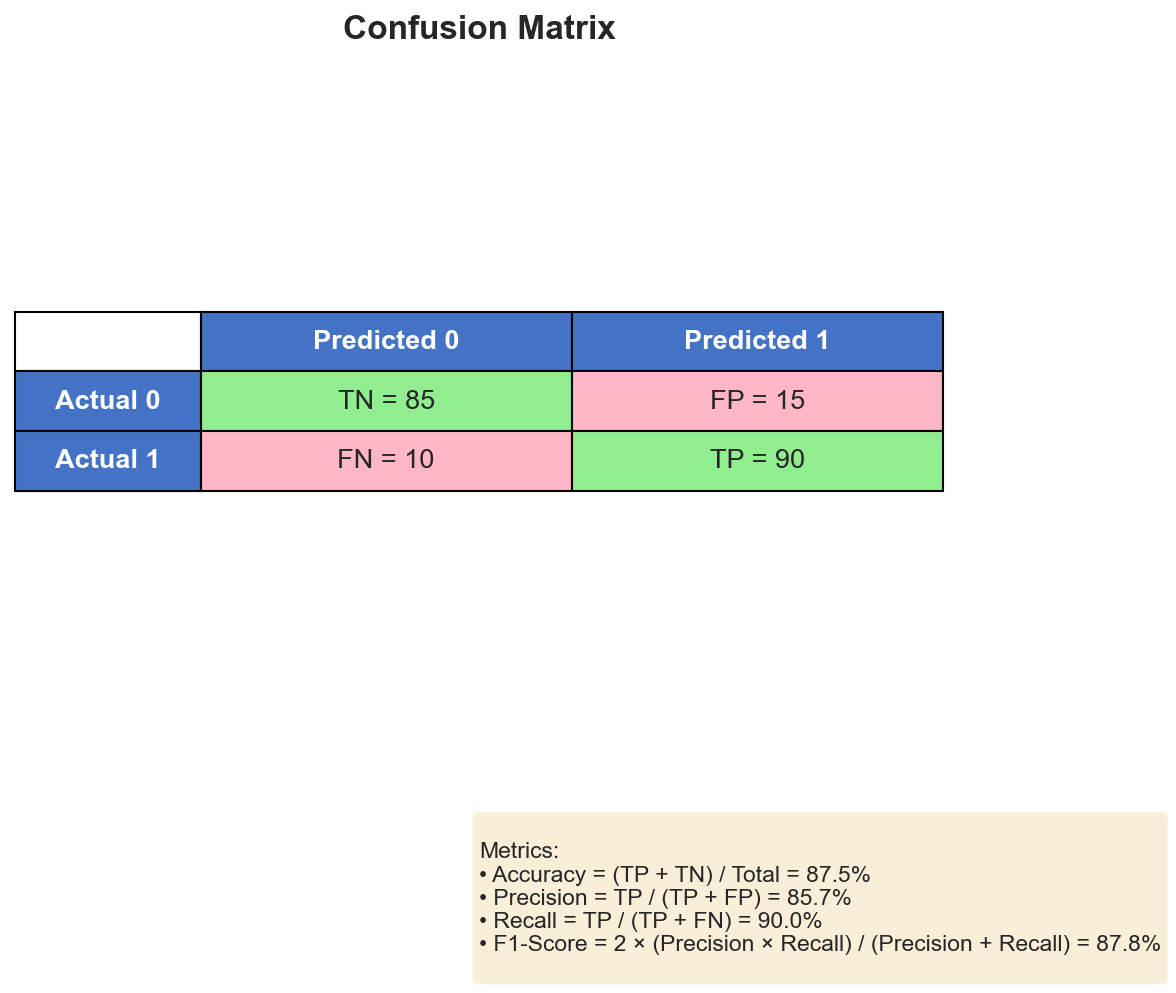
Confusion Matrix and Metrics
For classification tasks, we use:
| Predicted 0 | Predicted 1 | |
|---|---|---|
| Actual 0 | TN (True Neg) | FP (False Pos) |
| Actual 1 | FN (False Neg) | TP (True Pos) |
Metrics:
- Accuracy: \(\frac{TP + TN}{TP + TN + FP + FN}\)
- Precision: \(\frac{TP}{TP + FP}\)
- Recall (Sensitivity): \(\frac{TP}{TP + FN}\)
- Specificity: \(\frac{TN}{TN + FP}\)
- F1-Score: Harmonic mean of precision and recall
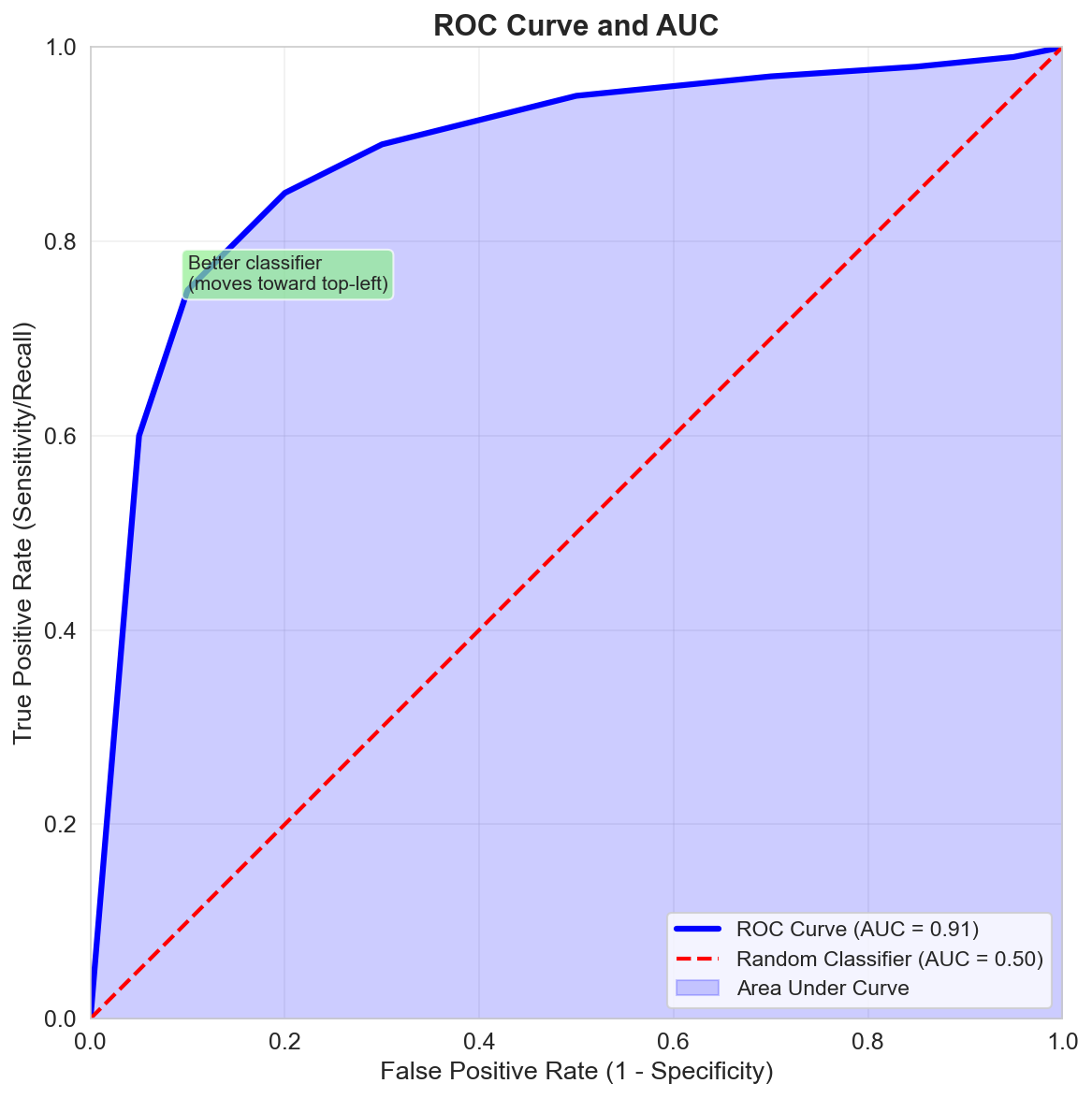
ROC Curve and AUC
The ROC curve (Receiver Operating Characteristic) plots True Positive Rate vs False Positive Rate at various threshold settings.
AUC (Area Under the Curve):
- \(AUC = 1\): Perfect classifier
- \(AUC = 0.5\): Random classifier
- \(AUC > 0.8\): Generally considered good
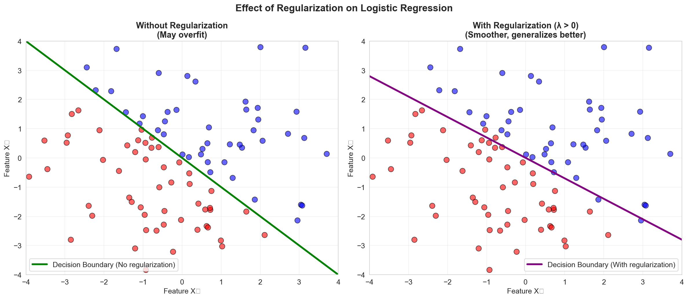
Regularization for Logistic Regression
Like linear regression, logistic regression can benefit from regularization when dealing with many predictors or collinearity.
L2 Regularization (Ridge)
\[ \text{NLL}(a) + \lambda \sum_{j=1}^{p} a_j^2 \]L1 Regularization (Lasso)
\[ \text{NLL}(a) + \lambda \sum_{j=1}^{p} |a_j| \]Benefits:
- Prevents overfitting
- Can perform variable selection (Lasso)
- Improves generalization to new data
Multiclass Logistic Regression
For \(K > 2\) classes, we use softmax regression (multinomial logistic regression).
The probability that observation \(i\) belongs to class \(k\) is:
\[ p_{ik} = P(Y_i = k \mid X_i) = \frac{\exp(\eta_{ik})}{\sum_{j=1}^{K} \exp(\eta_{ij})} \]where \(\eta_{ik} = a_k^T X_i\) for each class \(k\).
Training: Minimize the categorical cross-entropy loss:
\[ \text{Loss} = -\sum_{i=1}^{n} \sum_{k=1}^{K} \mathbb{1}(y_i = k) \log(p_{ik}) \]Summary
In this lesson we covered:
- ✅ Generalized Linear Models (GLM): extending beyond normal distributions
- ✅ Three components of a GLM: distribution, linear predictor, link function
- ✅ Logistic regression: binary classification using the logit link
- ✅ Maximum likelihood estimation: solving the negative log-likelihood
- ✅ Interpretation: odds, odds ratios, decision boundaries
- ✅ Model evaluation: confusion matrix, accuracy, precision, recall, ROC/AUC
- ✅ Regularization: Ridge and Lasso for logistic regression
- ✅ Multiclass extension: softmax regression
This completes the linear models series! You now have a solid foundation in:
- Simple and multiple linear regression
- Inference and diagnostics
- Feature engineering and polynomial regression
- Model selection and regularization
- GLMs and logistic regression for classification
Further Reading
- Generalized Additive Models (GAMs): Non-parametric extensions of GLMs
- Survival Analysis: Cox proportional hazards model
- Count Data: Poisson and negative binomial regression
- Hierarchical/Mixed Effects Models: Accounting for grouped/nested data structure