Introduction and Partitioning
Why Decision Trees?
Decision trees are supervised learning models used for both classification and regression. They are popular because they are easy to explain, can capture nonlinear behavior, and often need less manual feature engineering than linear models.
Three ideas make them especially attractive:
- Interpretability: a prediction can be read as a sequence of questions.
- Flexibility: trees can model interactions and nonlinear effects.
- Practicality: they work directly with mixed feature types and piecewise rules.
Tree Anatomy
A decision tree is built from three basic parts:
- An internal node tests a feature.
- A branch records the outcome of that test.
- A leaf stores the final prediction.
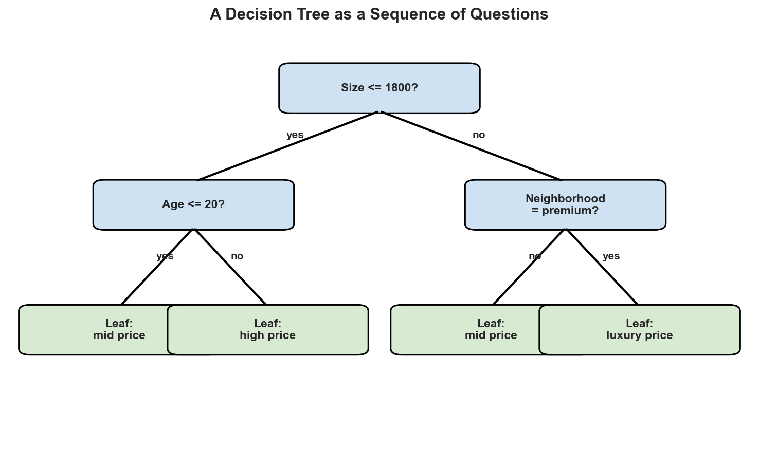
For classification, the leaf outputs a class. For regression, the leaf outputs a numeric value such as a local mean.
How Trees Partition the Feature Space
At each node, the tree chooses a feature \(x_j\) and a threshold \(t_j\), then splits the data into two regions:
\[ R_{\text{left}} = \{x : x_j \leq t_j\}, \qquad R_{\text{right}} = \{x : x_j > t_j\}. \]Applying this rule recursively creates a set of axis-aligned regions. Each leaf corresponds to one region of the feature space, so the tree behaves like a piecewise model.
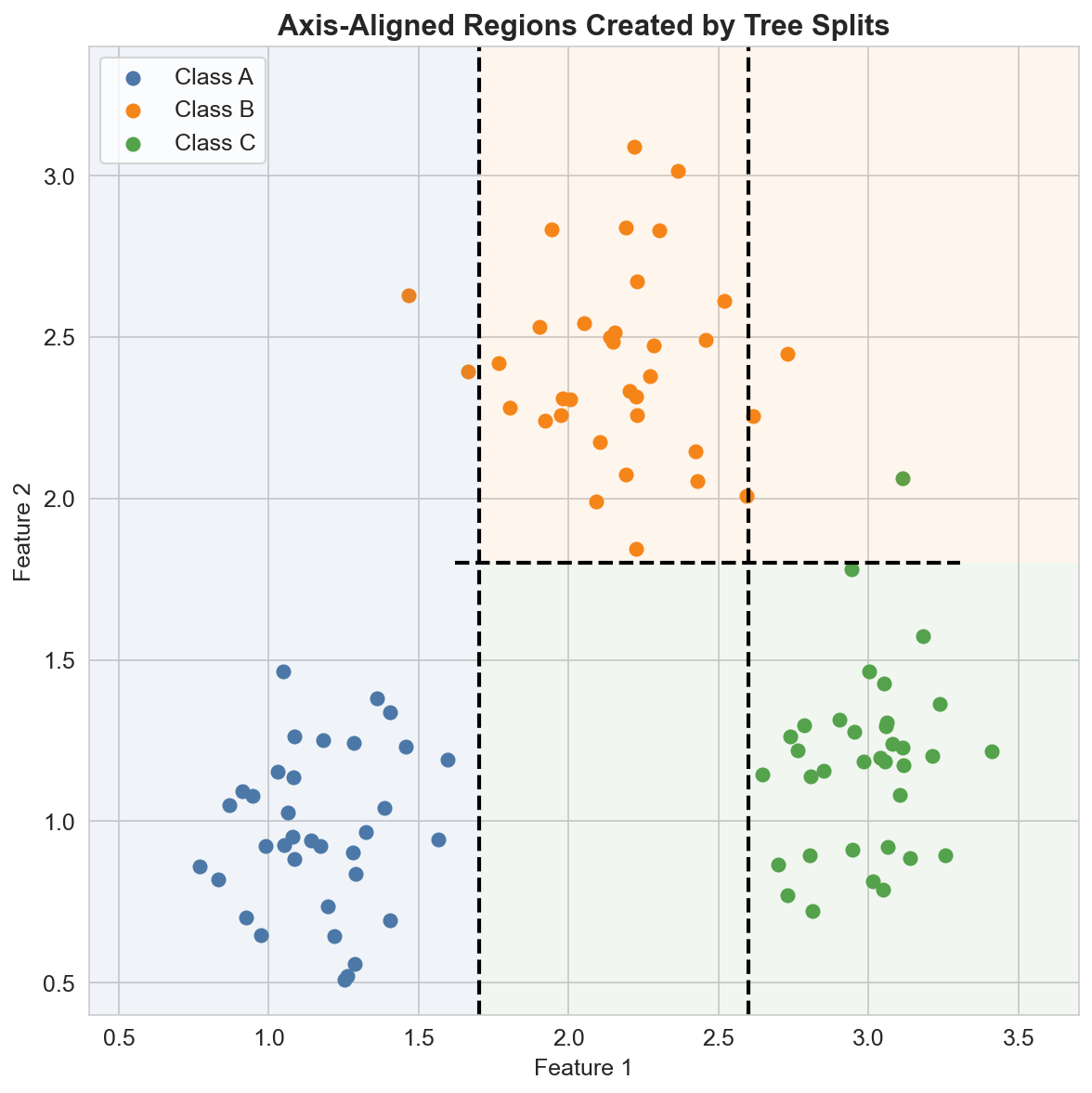
This is why trees can model nonlinear boundaries without writing interaction terms by hand.
What a Leaf Predicts
Suppose a classification tree creates regions \(R_1, \dots, R_M\). In a leaf \(R_m\), the empirical probability of class \(k\) is
\[ \hat{p}_{k \mid R_m} = \frac{1}{|R_m|}\sum_{x_i \in R_m} \mathbf{1}(y_i = k). \]When a new point \(x\) lands in region \(R_m\), the tree predicts the majority class:
\[ \hat{y}(x) = \arg\max_k \hat{p}_{k \mid R_m}. \]For regression, the same idea becomes a local average:
\[ \hat{y}(R_m) = \frac{1}{|R_m|}\sum_{x_i \in R_m} y_i. \]So a tree prediction is simple: find the leaf, then use the summary stored in that leaf.
Strengths and Typical Limits
Decision trees are strong first models when:
- you need a rule-based explanation,
- you expect interactions or threshold effects,
- or you want a model that is easy to visualize.
At the same time, a single tree can be unstable. A small change in the data may produce a different structure, which is why trees are considered high-variance models.
Summary
In this lesson we covered:
- The role of nodes, branches, and leaves in a decision tree
- How recursive splits partition the feature space into rectangular regions
- How classification leaves store class proportions
- How regression leaves store local average responses
- Why trees are both interpretable and sensitive to overfitting
Next: We will study how a tree chooses the best split using impurity criteria such as classification error, Gini, and entropy.