Splitting Criteria and Best Split
Why Split Quality Matters
At every internal node, a tree asks the same question:
Which feature and threshold produce the purest child nodes?
For classification, "pure" means that most observations in a node belong to the same class. A good split makes the left and right children more homogeneous than the parent node.
Classification Error
The simplest impurity measure is the classification error:
\[ \mathrm{Error}(R) = 1 - \max_k \hat{p}_{k \mid R}. \]If one class dominates the region, the error is small. If classes are mixed, the error is larger.
This criterion is easy to understand, but it is often not sensitive enough when comparing nearby candidate splits.
Gini Index
The Gini index is one of the most common criteria in classification trees:
\[ G(R) = 1 - \sum_{k=1}^{K} \hat{p}_{k \mid R}^2. \]For a binary problem with class proportion \(\hat{p}\), this becomes
\[ G(R) = 2\hat{p}(1-\hat{p}). \]The Gini index is:
- \(0\) for a perfectly pure node,
- largest when classes are evenly mixed,
- more sensitive than raw classification error.
Entropy
Another popular choice is entropy:
\[ H(R) = -\sum_{k=1}^{K} \hat{p}_{k \mid R}\log(\hat{p}_{k \mid R}). \]Like Gini, entropy is minimized when a node is pure and maximized when class proportions are close to uniform.
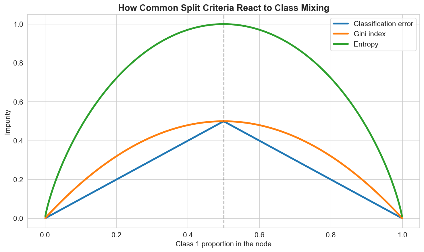
In practice:
- classification error is intuitive,
- Gini is efficient and widely used,
- entropy is slightly more aggressive in rewarding very pure splits.
Choosing the Best Split
Once an impurity measure \(I(R)\) is chosen, we score each candidate split \((j, t_j)\) by the impurity reduction:
\[ \Delta I(j, t_j) = I(R) - \left[ \frac{N_{\text{left}}}{N} I(R_{\text{left}}) + \frac{N_{\text{right}}}{N} I(R_{\text{right}}) \right]. \]Here:
- \(N\) is the number of samples in the parent node,
- \(N_{\text{left}}\) and \(N_{\text{right}}\) are the sizes of the child nodes.
We choose the split that maximizes \(\Delta I(j, t_j)\).
This is the tree analogue of asking: which local rule improves the node the most?
Handling Categorical Variables
Trees handle numerical variables naturally through threshold rules. With categorical variables, the goal is to divide the categories into two groups.
If a variable has \(C\) categories, the number of possible binary partitions is:
\[ 2^{C-1} - 1. \]That search can become expensive, so implementations often rely on heuristics or restricted search strategies. Some simple workflows encode categories numerically first, but that may introduce an artificial ordering that is not always meaningful.
Summary
In this lesson we covered:
- Why trees need impurity measures to compare candidate splits
- The definition of classification error
- The Gini index and its binary form
- Entropy as an alternative impurity criterion
- How impurity reduction defines the best split
- Why categorical predictors can make splitting more expensive
Next: We will see how stopping rules and pruning keep a tree from memorizing the training data.