Local Post-Hoc Methods
Explaining One Prediction at a Time
Local methods focus on a different question:
Why did the model produce this prediction for this specific input?
This is especially useful for debugging unusual cases, contesting decisions, or understanding failures on edge examples.
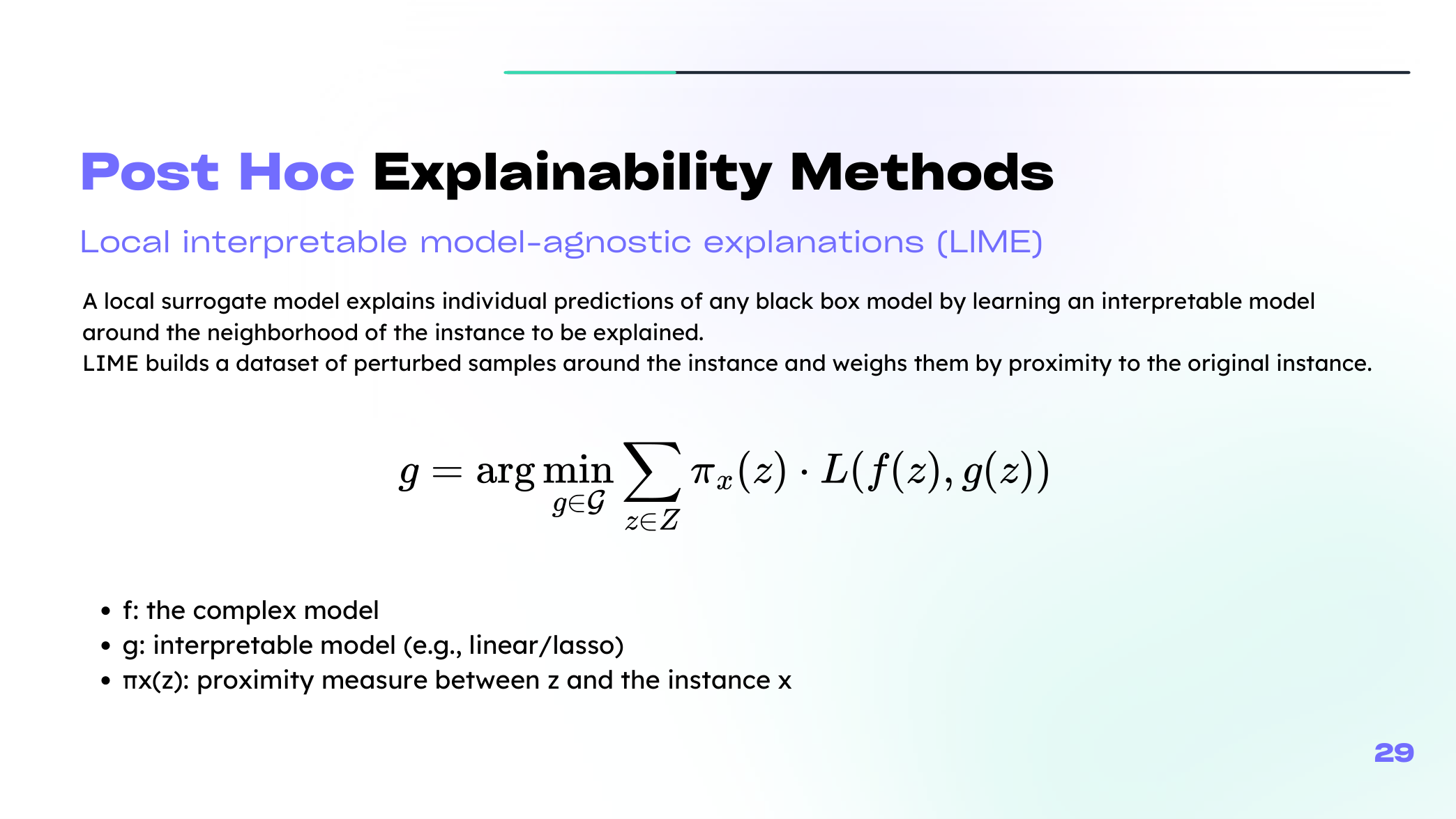
LIME
LIME builds a simple local surrogate around the instance we want to explain.
The core recipe is:
- perturb the input around the point of interest,
- query the black-box model on those perturbed samples,
- weight nearby samples more heavily,
- fit an interpretable model such as a sparse linear model.
In compact form, LIME solves a problem like
\[ \xi(x) = \arg\min_{g \in G} \; L\bigl(f, g, \pi_x\bigr) + \Omega(g), \]where \(g\) is a simple local model, \(\pi_x\) gives higher weight to points near \(x\), and \(\Omega(g)\) penalizes explanations that are too complex.
Your lecture shows how this idea changes across data types:
- for tabular data, we perturb feature values,
- for text, we remove or keep words,
- for images, we toggle superpixels on and off.
This is one of the places where the original slide still helps, because the neighborhood-and-surrogate idea is easier to grasp visually than verbally the first time.
LIME is intuitive and flexible, but it can be sensitive to the perturbation strategy and neighborhood definition.
From Shapley Values to SHAP
Shapley values come from cooperative game theory. They assign each feature a fair share of the prediction by averaging its marginal contribution across coalitions.
For feature \(j\), the Shapley value is
\[ \phi_j = \sum_{S \subseteq F \setminus \{j\}} \frac{|S|!(M-|S|-1)!}{M!} \Bigl(v(S \cup \{j\}) - v(S)\Bigr), \]where \(v(S)\) measures what the coalition \(S\) contributes to the prediction.
SHAP packages this idea into an additive explanation form:
\[ g(z') = \phi_0 + \sum_{j=1}^{M}\phi_j z'_j. \]Here, \(\phi_j\) represents the contribution of feature \(j\) to the prediction for the instance of interest.
KernelSHAP estimates these values by sampling coalitions and weighting them appropriately. It connects the local-surrogate spirit of LIME with the fairness logic of Shapley values.
| Method | Main output | Strength | Main caution |
|---|---|---|---|
| LIME | Sparse local surrogate | Very intuitive | Depends on perturbation design |
| SHAP | Additive feature attributions | Strong axiomatic basis | Can be expensive or assumption-heavy |
| Counterfactuals | Minimal change needed to flip the decision | Action-oriented | May suggest unrealistic edits |
| Anchors | Short sufficient rule | Easy to communicate | May miss broader model behavior |
Beyond LIME and SHAP
The lecture also places counterfactual explanations and anchors next to LIME and SHAP in the local-method family.
- Counterfactuals answer: "What small change would flip the prediction?"
- Anchors answer: "What short rule is sufficient to keep this prediction stable?"
They are valuable because they speak in slightly different languages: one is action-oriented, the other rule-oriented.
Reading Local Explanations Carefully
Local explanations are powerful, but they are not automatically faithful or stable.
We still have to ask:
- Is the perturbed neighborhood realistic?
- Would the explanation change a lot if we reran the method?
- Is the explanation aligned with domain knowledge?
That mindset matters as much as the method itself.
Summary
In this lesson we covered:
- Why local explanations focus on individual predictions
- How LIME builds a local surrogate
- How Shapley values lead to SHAP and KernelSHAP
- Why local explanations still need stability and realism checks
Next: We will study explainability tools that depend on the internal structure of trees and neural networks.